Week 4.1 - Genetic Algorithm

Explanation :

1. Program starts with clea rall, close all, clc.

2. Linspace command is used to define 150 x and y values between 0 to 0.6 with 50 iterations to run 50 times.

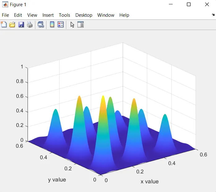
3. Meshgrid command is used to form 2D array.

4. For loop is executed to evaluate the stalagmite.

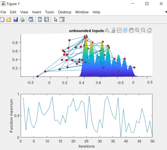
5. For case study1 - Statistical behaviour for loop is executed. During stalagmite function is called with 'ga'. Respectively plotting is done. Also tic and toc command is used to measure time taken for execution.

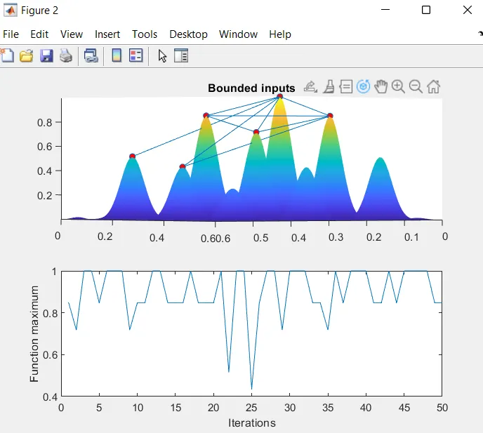
6. For case study2 - Statistical behaviour with upper and lower bounds, for loop is executed. During execution stalagmite function is called 'ga'. Also tic and toc commands is used to measure time taken for execution.

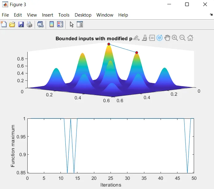
7. Again, for case study3 - With increasing iterations, for loop is executed. During execution stalagmite function is called 'ga'. Here optimoptions function is used to return ga solver and to define population size. Also tic and toc command is used to measure time taken for execution.

%Program for Stalagmite


clear all
close all
clc


%defining the search space
x= linspace(0,0.6,150);
y= linspace(0,0.6,150);
iterations= 50;

[xx yy]= meshgrid(x, y);


%stalagmite function
for i = 1:length(xx)
    for j = 1:length(yy)
        input_vector(1)=xx(i,j);
        input_vector(2)=yy(i,j);
        f(i,j) = stalagmite_func(input_vector);
    end
end

surf(xx,yy,-f)

xlabel('x value')
ylabel('y value')

shading interp

[x,fval] = ga(@stalagmite_func,2)

% 1st iteration- studying statistical behaviour
tic
for i = 1:iterations
    [inputs,fopt(i)] = ga(@stalagmite_func,2);
    xopt(i) = inputs(1);
    yopt(i) = inputs(2);
end

iteration1_time = toc
%plotting
figure(1)
subplot(2,1,1)
hold on 
surfc(xx,yy,-f)
shading interp
plot3(xopt,yopt,-fopt,'marker','o','markersize',5,'markerfacecolor','r')
title('unbounded inputs')
subplot(2,1,2)
plot(-fopt)
xlabel('iterations')
ylabel('Function maximum')

%2nd iteration with upper and lower limits

 tic
 for i = 1:iterations
 [inputs,fopt(i)] = ga(@stalagmite_func,2,[],[],[],[],[0;0],[1;1]);
 xopt(i) = inputs(1);
 yopt(i) = inputs(2);
 end
 iteration2_time =toc

 %plotting
 figure(2)
 subplot(2,1,1)
 hold on
 surfc(xx,yy,-f)
 shading interp
 plot3(xopt,yopt,-fopt,'marker','o','markersize',5,'markerfacecolor','r')
 title('Bounded inputs')
 subplot(2,1,2)
 plot(-fopt)
 xlabel('Iterations')
 ylabel('Function maximum')

 %3rd iteration- increasing the size of a population
 options = optimoptions('ga');
 options = optimoptions(options,'populationsize',200)

 tic
 for i = 1:iterations
     [inputs,fopt(i)] = ga(@stalagmite_func,2,[],[],[],[],[0;0],[1;1],[],[],options);
     xopt(i) = inputs(1);
     yopt(i) = inputs(2);
 end

 iterations3_time = toc
 %plotting
 figure(3)
 subplot(2,1,1)
 hold on
 surfc(xx,yy,-f)
 shading interp
 plot3(xopt,yopt,-fopt,'marker','o','markersize',5,'markerfacecolor','r')
 title('Bounded inputs with modified population size')
 subplot(2,1,2)
 plot(-fopt)
 xlabel('Iterations')
 ylabel('Function maximum')

%Function os stalagmite:

function [F] = stalagmite_func(input_vector)
x= input_vector(1);
y= input_vector(2);
f1= (sin(5.1*pi*x+0.5)).^6;
f2= (sin(5.1*pi*y+0.5)).^6;
f3= exp((-4*log(2)*(x-0.0667).^2)/(0.64));
f4= exp((-4*log(2)*(y-0.0667).^2)/(0.64));
F= -(f1*f2*f3*f4);
end

Output :

Unbounded inputs :

Bounded inputs :

Bounded inputs with modified population size :

Use of Genetic Alogorithm:

Fastest search technique.

Provide optimisation over large space state.

Does not require any derivation information.

Always gets an answer to the problem, which gets better over the time.

Useful when the search space is very large and there are a large number of parameters involved.

Make no assumption about the problem space.

Syntax of Ga:

x = ga(fun,nvars)

x = ga(fun,nvars,A,b)

x = ga(fun,nvars,A,b,Aeq,beq)

x = ga(fun,nvars,A,b,Aeq,beq,lb,ub)

x = ga(fun,nvars,A,b,Aeq,beq,lb,ub,nonIcon)

x = ga(fun,nvars,A,b,Aeq,beq,lb,ub,nonIcon,options)

x = ga(fun,nvars,A,b,[],[],lb,ub,nonIcon,IntCon)

x = ga(fun,nvars,A,b,[],[],lb,ub,nonIcon,IntCon,options)

x = ga(problem)

[x,fval] = ga(___)

[x,fval,exitflag,output] = ga(__)

[x,fval,exitflag,output,population,scores] = ga(__)

x = ga(problem) finds the minimum for problem, where problem is a structure.

[x,fval] = ga(__), for any previous input arguments also returns fval, the value of the fitness function at x.

Input arguments:

fun = objective function

nvars = number of variables

A- linear inequality constrains

b- linear inequality constrains

Aeq - linear equality constrains

beq - linear equality constrains

lb - lower bound

up - upper bound

nonIcon - Nonlinear constrains

options - linear variables

problem - problem descriptions

Output Arguments:

x - solution

fval - Objective function value at solution