Week 4.1 - Genetic Algorithm
Genetic Algorithm
Aim: To Write a code in MATLAB to optimise the stalagmite function and find the global maxima of the function.
Introduction:
Stalagmite : A stalagmite is a type of rock formation that rises from the floor of a cave due to the accumulation of material deposited on the floor from ceiling drippings. Stalagmites are typically composed of calcium carbonate,
We have mathematical function for Stalagmite,
`f(x,y) = fx1 * fx2 * fy1 * fy2`
Where , x and y are independent variables.
`fx1 = (sin(5.1*pi*x+ 0.5))^6`
`fy1 = (sin(5.1*pi*y + 0.5))^6`
`fx2 = exp(-(4*log(2)*(x - 0.0667)^2)/(0.64))`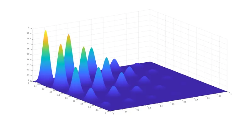
`fy2 = exp(-(4*log(2)*(y - 0.0667)^2)/(0.64))`
If we plot a graph for the above function with diffrent values of x and y show in the fig.
genetic algorithm:
Genetic Algorithm (GA) is a search-based optimization technique based on the principles of Genetics and Natural Selection. It is frequently used to find optimal or near-optimal solutions. It is frequently used to solve optimization problems, in research, and in machine learning.
In other words it is the random search based optimization algorithm for global minima of function by relying on biologically inspired operators such as mutation, crossover and selection.
Five stages in the genetic algorithm [2]
1. Initial population: the process begins with a set of individuals which is called a Population. Each individual is a solution to the problem you want to solve. the process begins with a set of individuals which is called a Population. Each individual is a solution to the problem you want to solve. Generally GA will take 50 as Population size if we are not specified. And we can change by modifying the GA.
2. Fitness function- It determines how to fit an individual is, in other words, it gives a fitness score to each individual.
3. Selection- In this phase it allows genes of fittest individuals to pass on to the next generation.
4. Crossover- It is the most significant phase in a genetic algorithm. For each pair of parents to be mated, a crossover point is chosen at random from within the genes.
5. Mutation- In certain new offsprings formed, some of them can be subjected to a mutation with a low random probability. This implies that some of the bits in the bit string can be flipped.
The following flowchart represents how a genetic algorithm works [1]
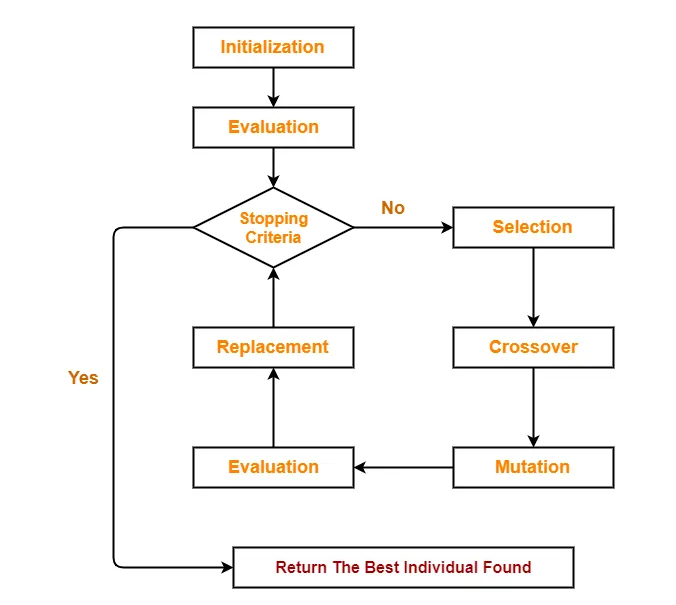
Stopping Criteria Options: Stopping criteria determine what causes the algorithm to terminate. You can specify the following options[4]
MaxGenerations — Specifies the maximum number of iterations for the genetic algorithm to perform. The default is 100*number O fVariables.
MaxTime — Specifies the maximum time in seconds the genetic algorithm runs before stopping, as measured by tic and toc. This limit is enforced after each iteration, so ga can exceed the limit when an iteration takes substantial time.
FitnessLimit — The algorithm stops if the best fitness value is less than or equal to the value of FitnessLimit. Does not apply to gamultiobj.
MaxStallGenerations — The algorithm stops if the average relative change in the best fitness function value over MaxStallGenerations is less than or equal to FunctionTolerance. (If the StallTest option is 'geometricWeighted', then the test is for a geometric weighted average relative change.) For a problem with nonlinear constraints, MaxStallGenerations applies to the subproblem (see Nonlinear Constraint Solver Algorithms). For gamultiobj, if the geometric average of the relative change in the spread of the Pareto solutions over MaxStallGenerations is less than FunctionTolerance, and the final spread is smaller than the average spread over the last MaxStallGenerations, then the algorithm stops. The geometric average coefficient is ½. The spread is a measure of the movement of the Pareto front. See gamultiobj Algorithm.
MaxStallTime — The algorithm stops if there is no improvement in the best fitness value for an interval of time in seconds specified by MaxStallTime, as measured by tic and toc.
FunctionTolerance — The algorithm stops if the average relative change in the best fitness function value over MaxStallGenerations is less than or equal to FunctionTolerance. (If the StallTest option is 'geometricWeighted', then the test is for a geometric weighted average relative change.) For gamultiobj, if the geometric average of the relative change in the spread of the Pareto solutions over MaxStallGenerations is less than FunctionTolerance, and the final spread is smaller than the average spread over the last MaxStallGenerations, then the algorithm stops. The geometric average coefficient is ½. The spread is a measure of the movement of the Pareto front. See gamultiobj Algorithm.
ConstraintTolerance — The ConstraintTolerance is not used as stopping criterion. It is used to determine the feasibility with respect to nonlinear constraints. Also, max(sqrt(eps),ConstraintTolerance) determines feasibility with respect to linear constraints. See Set Maximum Number of Generations and Stall Generations for an example.
Find minimum of function using genetic algorithm.
The following syntax can be used to perform GA [3].
1. x = ga(fun,nvars) finds a local unconstrained minimum, x, to the objective function, fun. nvars is the dimension (number of design variables) of fun.
2. x = ga(fun,nvars,A,b) finds a local minimum x to fun(function), subject to the linear inequalities A*x ≤ b. ga evaluates the matrix product A*x as if x is transposed (A*x').
3. x = ga(fun,nvars,A,b,Aeq,beq) finds a local minimum x to fun, subject to the linear equalities Aeq*x = beq and A*x ≤ b. (Set A=[] and b=[] if no linear inequalities exist.) ga evaluates the matrix product Aeq*x as if x is transposed (Aeq*x').
4. x = ga(fun,nvars,A,b,Aeq,beq) finds a local minimum x to fun, subject to the linear equalities Aeq*x = beq and A*x ≤ b. (Set A=[] and b=[] if no linear inequalities exist.) ga evaluates the matrix product Aeq*x as if x is transposed (Aeq*x').
5. x = ga(fun,nvars,A,b,Aeq,beq,lb,ub) defines a set of lower and upper bounds on the design variables, x, so that a solution is found in the range lb ≤ x ≤ ub. (Set Aeq=[] and beq=[] if no linear equalities exist.)
6. x = ga(fun,nvars,A,b,Aeq,beq,lb,ub,nonlcon) subjects the minimization to the constraints defined in nonlcon. The function nonlcon accepts x and returns vectors C and Ceq, representing the nonlinear inequalities and equalities respectively. ga minimizes the fun such that C(x) ≤ 0 and Ceq(x) = 0. (Set lb=[] and ub=[] if no bounds exist.)
7. x = ga(fun,nvars,A,b,Aeq,beq,lb,ub,nonlcon,options) minimizes with the default optimization parameters replaced by values in options. (Set nonlcon=[] if no nonlinear constraints exist.) Create options using optimoptions.
8. x = ga(fun,nvars,A,b,[],[],lb,ub,nonlcon,IntCon) or x = ga(fun,nvars,A,b,[],[],lb,ub,nonlcon,IntCon,options) requires that the variables listed in IntCon take integer values.
x = ga(fun,nvars,A,b,Aeq,beq,lb,ub,nonlcon,intcon,options)
Where, x = maximum value of resultant function
fun = fitness function
nvars = number of variables
A = linear inequality constraints, specified as real matrix A
b = linear inequality constraints, specified as real vector b
Aeq = linear equality constraints, specified as real matrix A
beq = linear equality constraints, specified as real vector b
lb = lower bound in search space of algorithm
ub = upper bound in search space of algorithm
nonlcon = non linear constraints
intcon = vector of positive integers
options = optimisation options
Function program
% creating stalagmite function
function [f] = stalagmite(input);

 % stalagmite function is given by f(x,y) = fx1 * fx2 * fy1 * fy2
 x = input(1);
 y = input(2);

 fx1 = (sin(5.1*pi*x+ 0.5))^6;
 fy1 = (sin(5.1*pi*y + 0.5))^6;
 fx2 = exp(-((4*log(2)*(x - 0.0667)^2)/(0.64)));
 fy2 = exp(-((4*log(2)*(y - 0.0667)^2)/(0.64)));

 [f] = -(fx1.*fx2.*fy1.*fy2);

  end
Program for problem:
1.Code for function for ploting:
Write code for generate surface plot of function by inputing the x and y values.
Define the search space data
x = linspace(0,0.6,150)
y = linspace(0,0.6,150)
create 2 data by using meshgrid
[xx, yy] = meshgrid(x,y)
for loop to reade data from created 2 data of xx
i = 1: length(xx) using foor loop to repeat the cycle for lenth times of xx meshgrid 150 times
for loop to reade data from created 2 data of yy for every value of xx
j = 1: length(yy) using foor loop to repeat the cycle for lenth times of y meshgrid 150 times
here 'j' loop will repeat 150 times for every 150 valuses of xx
input(1)= xx(i,j)
input(2)= yy(i,j)
F(i,j) = stalagmite(input); calling function for every value of xx and yy
plots.
figure(1)
surf(xx,yy,-F)
xlabel('X value')
ylabel('Y value')
title('stalagmite Function')
shading interp
Study -1 unbounded inputs, Running GA algorithm for 50 times.
for k = 1:iteration
in side ga (inside it reading values of function (Fval) randomly with 50 times And giving the values for x and y as input for for 50 times
[input, Fval(k)] = ga(@stalagmite,2), finds a local unconstrained minimum, inputs, to the objective function, fun. nvars is the dimension (number of design variables) of fun.
here the for loop will run 50 times and from the function GA will read minimum value of function then it will give values for inputs that is x and y. this genetic algorithm read randam data of function, and and i will give local minima. every run results will be different form each other.
x_out(k) = input(1) x_out(k) is storing randam value that algorithm will take for ploting purpose
y_out(k) = input(2) x_out(k) is storing randam value that algorithm will take for ploting purpose
end
study_1 = toc messuring run time
figure(2)
hold on
subplot(2,1,1) % subplot(rows,column, index) i.e here 2 rows, that is 2 plots are one below with first column and first index
surf(xx,yy,-F) % surface ploting, by inversing data,
xlabel('X value')
ylabel('Y value')
shading interp
hold on
plot3(x_out, y_out, -Fval,'marker','o','markersize',5,'markerfacecolor','r'), plot3 is used to connect points in 3d space.
title('Unbounded inputs')
subplot(2,1,2) subplot(rows,column, index) i.e here 2 rows meant 2 plots are one below with first column and 2nd index
plot(-Fval)
xlabel('Iteration')
ylabel('Function minimum')
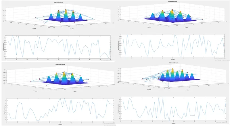
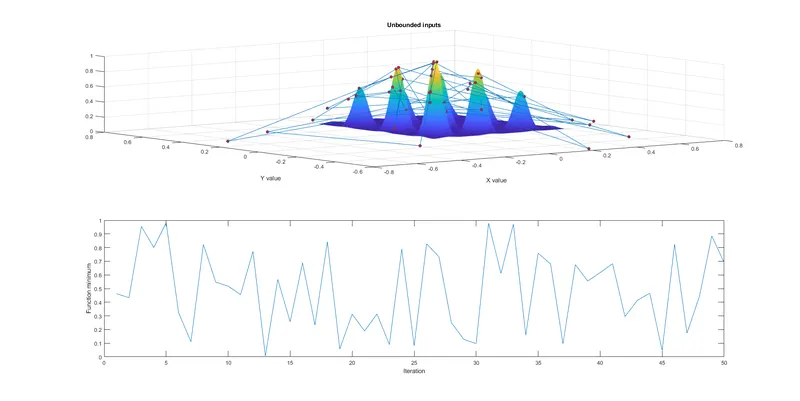
Similarly for
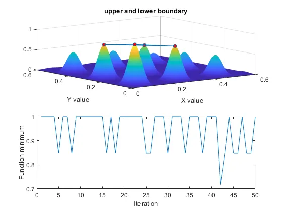
Study -2 Stastical behaviour upper and lower boundary.
[input, Fval(k)] = ga(@stalagmite,2,[],[],[],[],[0;0],[0.6;0.6]);
defines a set of lower and upper bounds on the design variables, inputs, so that a solution is found in the range lb( lower boun) ≤Inputs (x and y)≤ ub(upper bound). (Set Aeq=[] and beq=[] if no linear equalities exist.)
Here the for loop will runf 50 times and with in the bound for reading function data, compare to study its better,
iteration = 50;
tic
for k = 1:iteration;
% in side ga (inside it reading values of function (Fval) randomly with 50 times
% And giving the values for x and y as input for upper and lower boundaries
% boundaries x 0 to .6 abd y 0 to 0.6
[input, Fval(k)] = ga(@stalagmite,2,[],[],[],[],[0;0],[0.6;0.6]);
x_out(k) = input(1); % x_out(k) is storing randam value that algorithm will take for ploting purpose
y_out(k) = input(2); % x_out(k) is storing randam value that algorithm will take for ploting purpose
end
study_2 = toc
figure(3)
hold on
subplot(2,1,1) % subplot(rows,column, index) i.e here 2 rows meant 2 plots are one below with first column and first index
surf(xx,yy,-F) % surface ploting
xlabel('X value')
ylabel('Y value')
shading interp
hold on
plot3(x_out, y_out, -Fval,'marker','o','markersize',5,'markerfacecolor','r')
title('upper and lower boundary')
subplot(2,1,2)
plot(-Fval)
xlabel('Iteration')
ylabel('Function minimum')
Similarly for
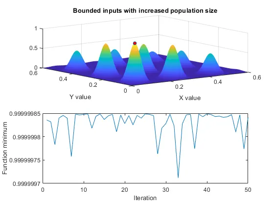
Study -3 Stastical behaviour of upper and lower bounds with increased GA
[input, Fval(k)] = ga(@stalagmite,2,[],[],[],[],[0;0],[0.6;0.6],[],[],options)
minimizes with the default optimization parameters replaced by values in options. (Set nonlcon=[] if no nonlinear constraints exist.) Create options using optimoptions.
here increasing populationsize from default 50 to 190. ga will place 190 random points with in the bound and reads function value. so that every time i will same results. but time taken to compute is more than other 2 studies.
optimoptions: Create optimization options
options = optimoptions(SolverName); here slover name si ga (genetic algorithm)
options = optimoptions(SolverName,Name,Value); Name is populationsize, val is 190,
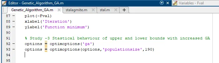
options = optimoptions('ga')
options = optimoptions(ga,'populationsize',190), here increasing populationsize from default 50 to 190.
tic
for k = 1:iteration;
% in side ga (inside it reading values of function (Fval) randomly with 50 times
% And giving the values for x and y as input for upper and lower boundaries
% boundaries x 0 to .6 abd y 0 to 0.6
[input, Fval(k)] = ga(@stalagmite,2,[],[],[],[],[0;0],[0.6;0.6],[],[],options);
%x = ga(fun,nvars,A,b,[],[],lb,ub,nonlcon,IntCon,options)
x_out(k) = input(1); % x_out(k) is storing randam value that algorithm will take for ploting purpose
y_out(k) = input(2); % x_out(k) is storing randam value that algorithm will take for ploting purpose
end
study_3 = toc
figure(4)
hold on
subplot(2,1,1) % subplot(rows,column, index) i.e here 2 rows meant 2 plots are one below with first column and first index
surf(xx,yy,-F) % surface ploting
xlabel('X value')
ylabel('Y value')
shading interp
hold on
plot3(x_out, y_out, -Fval,'marker','o','markersize',5,'markerfacecolor','r')
title('Bounded inputs with increased population size')
subplot(2,1,2)
plot(-Fval)
xlabel('Iteration')
ylabel('Function minimum')
%Write a code in MATLAB to optimise the stalagmite function and find the global maxima of the function.
close all
clear all
clc

% Define the search space data
x = linspace(0,0.6,150);
y = linspace(0,0.6,150);

% create 2 data by using meshgrid
[xx, yy] = meshgrid(x,y);

for i = 1: length(xx)  % using foor loop to repeat the cycle for lenth times of xx meshgrid 150 times

    for j = 1: length(yy) %% using foor loop to repeat the cycle for lenth times of y meshgrid 150 times
     % here 'j' loop will repeat 150 times for every 150 valuses of xx
     input(1)= xx(i,j);
     input(2)= yy(i,j);

     F(i,j) = stalagmite(input); % calling function for every value of xx and yy
    end
end

figure(1)
surf(xx,yy,-F)
xlabel('X value')
ylabel('Y value')
title('stalagmite Function')
shading interp


% Study -1 unbounded inputs, Running GA algorithm for 50 times.

iteration = 50;
tic
for k = 1:iteration;
    % in side ga (inside it reading values of function (Fval) randomly with 50 times
     % And giving the values for x and y as input for for 50 times
[input, Fval(k)] = ga(@stalagmite,2);
x_out(k) = input(1);                      % x_out(k) is storing randam value that algorithm will take for ploting purpose
y_out(k) = input(2);                     % x_out(k) is storing randam value that algorithm will take for ploting purpose
end
study_1 = toc

figure(2)
hold on
subplot(2,1,1)              % subplot(rows,column, index) i.e here 2 rows meant 2 plots are one below with first column and first index
surf(xx,yy,-F)                % surface ploting
xlabel('X value')
ylabel('Y value')
shading interp
hold on
plot3(x_out, y_out, -Fval,'marker','o','markersize',5,'markerfacecolor','r')
title('Unbounded inputs')
subplot(2,1,2)
plot(-Fval)
xlabel('Iteration')
ylabel('Function minimum')


% Study -2 Stastical behaviour upper and lower boundary.

iteration = 50;
tic
for k = 1:iteration;
    % in side ga (inside it reading values of function (Fval) randomly with 50 times
     % And giving the values for x and y as input for upper and lower boundaries
     % boundaries x 0 to .6 abd y 0 to 0.6
[input, Fval(k)] = ga(@stalagmite,2,[],[],[],[],[0;0],[0.6;0.6]);
x_out(k) = input(1);                      % x_out(k) is storing randam value that algorithm will take for ploting purpose
y_out(k) = input(2);                     % x_out(k) is storing randam value that algorithm will take for ploting purpose
end
study_2 = toc

figure(3)
hold on
subplot(2,1,1)              % subplot(rows,column, index) i.e here 2 rows meant 2 plots are one below with first column and first index
surf(xx,yy,-F)                % surface ploting
xlabel('X value')
ylabel('Y value')
shading interp
hold on
plot3(x_out, y_out, -Fval,'marker','o','markersize',5,'markerfacecolor','r')
title('upper and lower boundary')
subplot(2,1,2)
plot(-Fval)
xlabel('Iteration')
ylabel('Function minimum')

% Study -3 Stastical behaviour of upper and lower bounds with increased GA
options = optimoptions('ga')
options = optimoptions(options,'populationsize',190)

tic
for k = 1:iteration;
    % in side ga (inside it reading values of function (Fval) randomly with 50 times
     % And giving the values for x and y as input for upper and lower boundaries
     % boundaries x 0 to .6 abd y 0 to 0.6
[input, Fval(k)] = ga(@stalagmite,2,[],[],[],[],[0;0],[0.6;0.6],[],[],options);
%x = ga(fun,nvars,A,b,[],[],lb,ub,nonlcon,IntCon,options)
x_out(k) = input(1);                      % x_out(k) is storing randam value that algorithm will take for ploting purpose
y_out(k) = input(2);                     % x_out(k) is storing randam value that algorithm will take for ploting purpose
end
study_3 = toc

figure(4)
hold on
subplot(2,1,1)              % subplot(rows,column, index) i.e here 2 rows meant 2 plots are one below with first column and first index
surf(xx,yy,-F)                % surface ploting
xlabel('X value')
ylabel('Y value')
shading interp
hold on
plot3(x_out, y_out, -Fval,'marker','o','markersize',5,'markerfacecolor','r')
title('Bounded inputs with increased population size')
subplot(2,1,2)
plot(-Fval)
xlabel('Iteration')
ylabel('Function minimum')
Results: Write a code in MATLAB to optimise the stalagmite function and find the global maxima of the function so that code gives the same output, even if it is made to run several times is done.
we fund from all 3 studies
1. Genetic algorithm read randam data of function, and and i will give local minima. every run results were different form each other.
2. Genetic algorithm read randam data of function, and and i will give local minima. every run, some results were same and some results different form each other.
3. results were same for every run. Fval is 0.99 and time taken to compute is 24.75s.
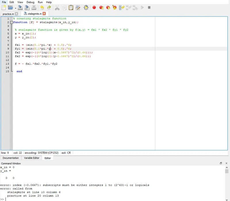
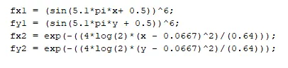
Errors:
1. improper function equations
2. not defined options
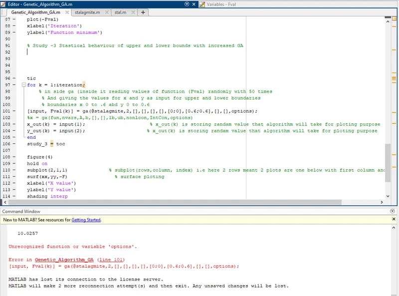
Reference:
[1 ]https://www.gatevidyalay.com/genetic-algorithm-in-ai-operators-working/
[2] https://skill-lync.com/knowledgebase/genetic-algorithm-explained
[3] https://in.mathworks.com/help/gads/ga.html
[4] https://in.mathworks.com/help/gads/genetic-algorithm-options.html#f14223