Week 4.1 - Genetic Algorithm
AIM- To Write a code in MATLAB to optimise the stalagmite function and find the global maxima of the function.
Theory
Genetic Algorithm (GA) is a search-based optimization technique based on the principles of Genetics and Natural Selection. It is frequently used to find optimal or near-optimal solutions to difficult problems which otherwise would take a lifetime to solve. It is frequently used to solve optimization problems, in research, and in machine learning.
Introduction to Optimization
Optimization is the process of making something better. In any process, we have a set of inputs and a set of outputs as shown in the following figure.
Inputs Process Outputs
Optimization refers to finding the values of inputs in such a way that we get the "best" output values. The definition of "best" varies from problem to problem, but in mathematical terms, it refers to maximizing or minimizing one or more objective functions, by varying the input parameters.
Main Program
clear all
close all
clc
% Defining our surch space
x = linspace(0,0.6,150);
y = linspace(0,0.6,150);
num_cases = 50
% creating a 2dimensional mesh
[xx yy]= meshgrid(x,y);
%evaluatin of stalagmite function
for i = 1:length(xx)
for j = 1:length(yy)
input_vector(1)=xx(i,j);
input_vector(2)=yy(i,j);
GA(i,j) = stalagmite(input_vector);
end
end
% study 1 |Statistical behaviour In unbounded condition
%tic_toc command for ireration
tic
for i = 1:num_cases
[input,GA_opt(i)]=ga(@stalagmite,2);
xopt(i)= input(1);
yopt(i)= input(2);
end
study_1_time = toc
% ploting the graph
figure (1)
subplot(2,1,1)
hold on
surfc(xx,yy,GA)
shading interp
plot3(xopt,yopt,GA_opt,'marker','o','markersize',5,'markerfacecolor','r');
title('Unbounded Inputs')
subplot(2,1,2)
plot(GA_opt)
xlabel('Iteration')
ylabel('Function minimum')
% study 2 |Statistical behaviour - upper & Lower bond
tic
for i = 1:num_cases
[input,GA_opt(i)]=ga(@stalagmite,2,[],[],[],[],[0;0],[1;1]);
xopt(i)= input(1);
yopt(i)= input(2);
end
study_2_time = toc
% ploting the graph
figure (2)
subplot(2,1,1)
hold on
surfc(xx,yy, GA)
shading interp
plot3(xopt,yopt, GA_opt, 'marker','o','markersize',5,'markerfacecolor','r');
title('Bounded Input')
subplot(2,1,2)
plot(GA_opt)
xlabel('Iteration')
ylabel('Function minimun')
% study 2 |Increasing GA Iterations
options = optimoptions('ga');
options = optimoptions(options,'populationsize',200);
tic
for i = 1:num_cases
[input,GA_opt(i)]=ga(@stalagmite,2,[],[],[],[],[0;0],[1;1],[],[],options);
xopt(i)= input(1);
yopt(i)= input(2);
end
study_3_time = toc
% ploting the graph
figure(3)
subplot(2,1,1)
hold on
surfc(xx,yy, GA)
shading interp
plot3(xopt,yopt, GA_opt, 'marker','o','markersize',5,'markerfacecolor','r');
title('Bounded Inputs with modified population size')
subplot(2,1,2)
plot(GA_opt)
xlabel('Iteration')
ylabel('Function minimun')
[x fval]=ga(@stalagmite,2)
% calulating function GA-Ganetic algorithe -stalagmite function.
function[GA]= stalagmite(input_vector)
x=input_vector(1);
y=input_vector(2);
unit1 = pi*5.1*x;
unit2 = pi*5.1*y;
unit3 = ((x-0.0667)^2/0.64);
unit4 = ((y-0.0667)^2/0.64);
unit5 = (-4)*log(2);
f1x = (sin(unit1+0.5))^6;
f1y = (sin(unit2+0.5))^6;
f2x = exp(unit5*unit3);
f2y = exp(unit5*unit4);
GA = -(f1x*f1y*f2x*f2y);
end
Program - code and plot explanation
clear all
close all
clc
% Defining our surch space
x = linspace(0,0.6,150);
y = linspace(0,0.6,150);
num_cases = 50
Value of x and y taking 150 values between the 0 to 0.6
We consider no of iteration num_cases=50
% creating a 2dimensional mesh
[xx yy]= meshgrid(x,y);
%evaluatin of stalagmite function
for i = 1:length(xx)
for j = 1:length(yy)
input_vector(1)=xx(i,j);
input_vector(2)=yy(i,j);
GA(i,j) = stalagmite(input_vector);
GA is only minimize a given function, Is considered it automatically gives the maxima.
end
end
% study 1 |Statistical behaviour In unbounded condition
%tic_toc command for ireration
tic
for i = 1:num_cases
[input,GA_opt(i)]=ga(@stalagmite,2);
xopt(i)= input(1);
yopt(i)= input(2);
end
study_1_time = toc
% ploting the graph
figure (1)
subplot(2,1,1)
hold on
surfc(xx,yy,GA)
shading interp
plot3(xopt,yopt,GA_opt,'marker','o','markersize',5,'markerfacecolor','r');
title('Unbounded Inputs')
subplot(2,1,2)
plot(GA_opt)
xlabel('Iteration')
ylabel('Function minimum')
we store the xopt,yopt,GA_opt. now we need to plot the surface xx,yy,GA to gate 3D plot
used command to make a plot of xopt,yopt,GA_opt to plot of optimum maximas.
Also tic-toc command used to record the time
Output
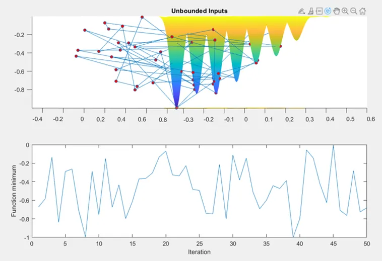
We can see the optimal values went outside the value of x and y and result is in falling away from the stalagmite surface
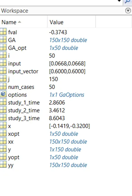
The study time is 2.8606s
% study 2 |Statistical behaviour - upper & Lower bond
tic
for i = 1:num_cases
[input,GA_opt(i)]=ga(@stalagmite,2,[],[],[],[],[0;0],[1;1]);
xopt(i)= input(1);
yopt(i)= input(2);
end
study_2_time = toc
% ploting the graph
figure (2)
subplot(2,1,1)
hold on
surfc(xx,yy, GA)
shading interp
plot3(xopt,yopt, GA_opt, 'marker','o','markersize',5,'markerfacecolor','r');
title('Bounded Input')
subplot(2,1,2)
plot(GA_opt)
xlabel('Iteration')
ylabel('Function minimun')
Output
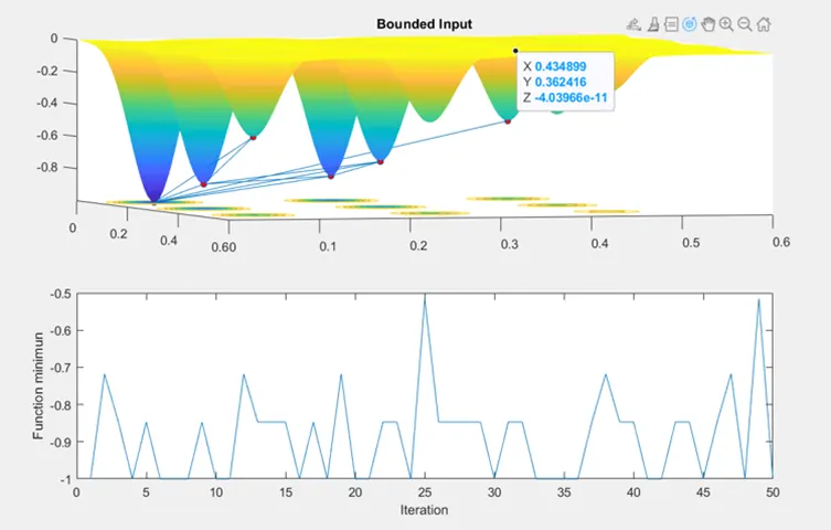
Study time is 3.4612s
% study 3 |Increasing GA Iterations
options = optimoptions('ga');
options = optimoptions(options,'populationsize',200);
tic
for i = 1:num_cases
[input,GA_opt(i)]=ga(@stalagmite,2,[],[],[],[],[0;0],[1;1],[],[],options);
xopt(i)= input(1);
yopt(i)= input(2);
end
study_3_time = toc
% ploting the graph
figure(3)
subplot(2,1,1)
hold on
surfc(xx,yy, GA)
shading interp
plot3(xopt,yopt, GA_opt, 'marker','o','markersize',5,'markerfacecolor','r');
title('Bounded Inputs with modified population size')
subplot(2,1,2)
plot(GA_opt)
xlabel('Iteration')
ylabel('Function minimun')
Output
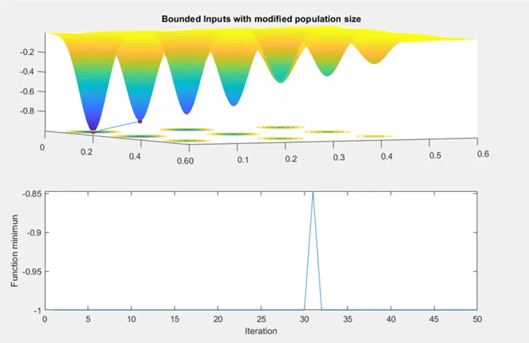
The study time is -8.6043 wiich is more than above two studies
[x fval]=ga(@stalagmite,2)
% calulating function GA-Ganetic algorithem
function[GA]= stalagmite(input_vector)
x=input_vector(1);
y=input_vector(2);
unit1 = pi*5.1*x;
unit2 = pi*5.1*y;
unit3 = ((x-0.0667)^2/0.64);
unit4 = ((y-0.0667)^2/0.64);
unit5 = (-4)*log(2);
f1x = (sin(unit1+0.5))^6;
f1y = (sin(unit2+0.5))^6;
f2x = exp(unit5*unit3);
f2y = exp(unit5*unit4);
GA = -(f1x*f1y*f2x*f2y);
end
Take number of iteration = num_cases and used genetic algorithm function to calculate the maxima of the function