Week 4.1 - Genetic Algorithm

Aim:-To Write a code in MATLAB to optimize the stalagmite function and also the globle maxima of the function.

Genetic Algotithm:- GA is the process of natural selection starts with the selection of fittest individuals from a population. They produce offspring which inherit the characteristics of the parents and will be added to the next generation. If parents have better fitness, their offspring will be better than parents and have a better chance at surviving. This process keeps on iterating and at the end, a generation with the fittest individuals will be found.

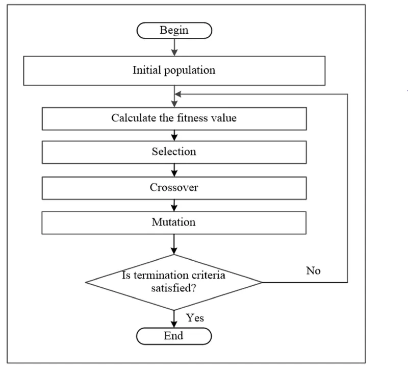
Five phases are considered in a genetic algorithm.

1. Initial population
2. Fitness function
3. Selection
4. Crossover
5. Mutation

Stalagamite Function used in program

Three cased perform in the code:

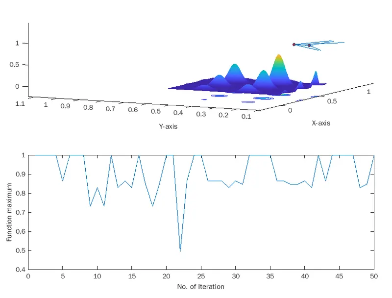
1. Unbounded inputs.

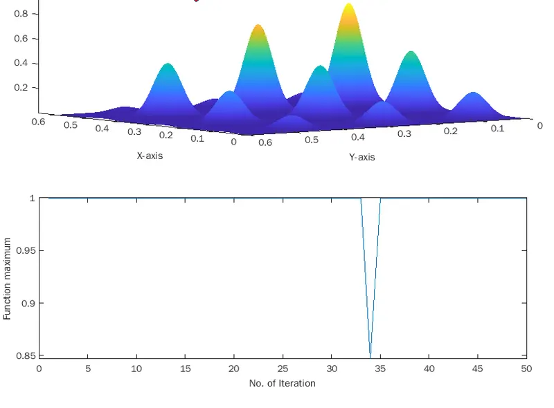
2. Bounded inputs restricted with upper and lower bounds

3. Bounded inputs with options increasing no of iteration by giving population size.

MATLAB code:-

1. Stalagmite function

2.Genetic Algorithm

clear all

close all

clc

x = linspace(0,0.6,150)

y = linspace(0,0.6,150)

n=50;

%Creating 2D mesh

[xx, yy] = meshgrid(x,y);

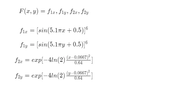
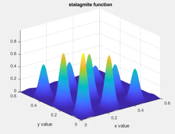
%stalagmite function

for i= 1:length(xx)

for j= 1:length(yy)

input_vector(1)=xx(i,j);

input_vector(2)=yy(i,j);

f(i,j) = stalagmite(input_vector);

end

end

%Study 1 : Statistical Behaviour

tic

for i= 1:n

[inputs,fopt(i)] = ga(@stalagmite,2);

xopt(i) = inputs(1);

yopt(i) = inputs(2);

end

study1_time =toc

figure(1)

subplot(2,1,1)

hold on

surfc(xx, yy,-f)

shading interp

xlabel('X-axis')

ylabel('Y-axis')

title('Statistical Behaviour with Unbound inputs')

plot3(xopt,yopt,-fopt,'marker','o','markersize',5,'markerfacecolor','r');

subplot(2,1,2);

plot(-fopt)

xlabel('No. of Iteration')

ylabel('Function maximum')

%Study2 : Statistical behaviour with upper and lower bound

tic

for i= 1:n

[inputs,fopt(i)] = ga(@stalagmite,2,[],[],[],[],[0;0],[1,1]);

xopt(i) = inputs(1);

yopt(i) = inputs(2);

end

study2_time =toc

figure(2)

subplot(2,1,1)

hold on

surfc(xx, yy,-f)

shading interp

xlabel('X-axis')

ylabel('Y-axis')

title('Statistical Behaviour with Unbound inputs')

plot3(xopt,yopt,-fopt,'marker','o','markersize',5,'markerfacecolor','r');

subplot(2,1,2);

plot(-fopt)

xlabel('No. of Iteration')

ylabel('Function maximum')

%Study3 : Statistical Behaviour with increasing iteration of ga

options = optimoptions('ga')

options = optimoptions(options,'PopulationSize',300)

tic

for i= 1:n

[inputs,fopt(i)] = ga(@stalagmite,2,[],[],[],[],[0;0],[1;1],[],[],options);

xopt(i) = inputs(1);

yopt(i) = inputs(2);

end

study3_time =toc

figure(3)

subplot(2,1,1)

hold on

surfc(xx, yy,-f)

shading interp

xlabel('X-axis')

ylabel('Y-axis')

title('Statistical Behaviour with Unbound inputs')

plot3(xopt,yopt,-fopt,'marker','o','markersize',5,'markerfacecolor','r');

subplot(2,1,2);

plot(-fopt)

xlabel('No. of Iteration')

ylabel('Function maximum')

Code Explanation:-

1. Linspace used to set the range of data between two points

2. meshgride command is used to create an array.

3. surfc(x,y,z) to create three dimensional surface plot

4. (lable) used to define the axis.

5. (shading interp) is used to hide the grid plot and smooth the plot.

Results:-

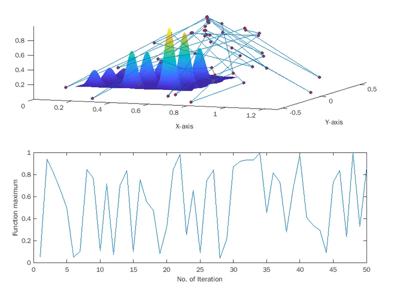
1. Unbounded inputs.

2.Bounded inputs restricted with upper and lower bounds

3. Bounded inputs with options increasing no of iteration by giving population size.

Used Links:-

1) in.mathworks.com/help/gads/constrained-minimization-using-ga.html;jsessionid=ddcab08c4e880e9863ca88292567

2) https://in.mathworks.com/discovery/genetic-algorithm.html