Week 4.1 - Genetic Algorithm
AIM:
To write a code in MATLAB to optimise the stalagmite function and find the global maxima of the function.
INTRODUCTION:
A stalagmite is a type of rock formation that rises from the floor of a cave due to the accumulation of material deposited on the floor from ceiling drippings.
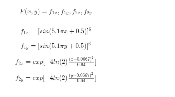
A stalagmite function generally refers to the function with which we are generating values over a stalagmite kind of surface for finding out the local and global maxima and minima of that particular given function.
FORMULAE:
FUNCTION CODE:
function [f]= stalagmite(input_vector)

x = input_vector(1);
y = input_vector(2);

%formula given
f1x = (sin((5.1*pi*x)+ 0.5)).^6;
f2y= (sin((5.1*pi*y)+0.5)).^6;
f3x = exp((-4*log(2)).*(x-0.0667)^2/(0.64));
f4y = exp((-4*log(2)).*(y-0.0667)^2/(0.64));
f = -(f1x*f2y*f3x*f4y);

end
GENETIC ALGORITHM:
A genetic algorithm (GA) is a method for solving both constrained and unconstrained optimization problems based on a natural selection process that mimics biological evolution. The algorithm repeatedly modifies a population of individual solutions. At each step, the genetic algorithm randomly selects individuals from the current population and uses them as parents to produce the children for the next generation. Over successive generations, the population "evolves" toward an optimal solution.
WORKING OF GENETIC ALGORITHM:
The following outline summarizes how the genetic algorithm works:
-
The algorithm begins by creating a random initial population.
-
The algorithm then creates a sequence of new populations. At each step, the algorithm uses the individuals in the current generation to create the next population. To create the new population, the algorithm performs the following steps:
-
Scores each member of the current population by computing its fitness value. These values are called the raw fitness scores.
-
Scales the raw fitness scores to convert them into a more usable range of values. These scaled values are called expectation values.
-
Selects members, called parents, based on their expectations.
-
Some of the individuals in the current population that have lower fitness are chosen as elite. These elite individuals are passed to the next population.
-
Produces children from the parents. Children are produced either by making random changes to a single parent—mutation—or by combining the vector entries of a pair of parents—crossover.
-
Replaces the current population with the children to form the next generation.
-
-
The algorithm stops when one of the stopping criteria is met.
-
The algorithm takes modified steps for linear and integer constraints.
-
The algorithm is further modified for nonlinear constraints.
CREATING NEXT GENERATION:
The genetic algorithm creates three types of children for the next generation:
-
Elite are the individuals in the current generation with the best fitness values. These individuals automatically survive to the next generation.
-
Crossover is created by combining the vectors of a pair of parents.
-
Mutation children are created by introducing random changes, or mutations, to a single parent.
The following schematic diagram illustrates the three types of children.
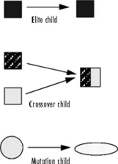
Mutation and Crossover explains how to specify the number of children of each type that the algorithm generates and the functions it uses to perform crossover and mutation.
Crossover Children
The algorithm creates crossover children by combining pairs of parents in the current population. At each coordinate of the child vector, the default crossover function randomly selects an entry, or gene, at the same coordinate from one of the two parents and assigns it to the child. For problems with linear constraints, the default crossover function creates the child as a random weighted average of the parents.
Mutation Children
The algorithm creates mutation children by randomly changing the genes of individual parents. By default, for unconstrained problems, the algorithm adds a random vector from a Gaussian distribution to the parent. For bounded or linearly constrained problems, the child remains feasible.
SYNTAX:
x = ga(fun,nvars,A,b,Aeq,beq,lb,ub)x, so that a solution is found in the range lb ≤ x ≤ ub. (Set Aeq=[] and beq=[] if no linear equalities exist.)
x = ga(fun,nvars,A,b,Aeq,beq,lb,ub,nonlcon)nonlcon. The function nonlcon accepts x and returns vectors C and Ceq, representing the nonlinear inequalities and equalities respectively. ga minimizes the fun such that C(x) ≤ 0 and Ceq(x) = 0. (Set lb=[] and ub=[] if no bounds exist.)
x = ga(fun,nvars,A,b,Aeq,beq,lb,ub,nonlcon,options)options. (Set nonlcon=[] if no nonlinear constraints exist.) Create options using optimoptions.
[ also returns a matrix x,fval,exitflag,output,population,scores] = ga(___)population, whose rows are the final population, and a vector scores, the scores of the final population.
Where,
nvars |
Number of design variables |
Aineq |
|
Bineq |
|
Aeq |
|
Beq |
|
lb |
Lower bound on |
ub |
Upper bound on |
nonlcon |
Nonlinear constraint functions |
solver |
|
options |
Options created using |
CODE TO FIND GLOBAL MAXIMA:
close all
clear all
clc

%inputs
x = linspace(0,0.6,150);
y = linspace(0,0.6,150);
% no of iterations
n = 50;

%creating  2D
[xx,yy] = meshgrid(x,y);

%stalagamite code
tic
for i = 1:length(xx)
    for j = 1:length(yy)
        input_vector(1)= xx(i,j);
        input_vector(2)= yy(i,j);
        f(i,j)= stalagmite(input_vector);
    end
end
studytime = toc

figure(1)
surfc(xx,yy,-f)
shading interp
xlabel('x value')
ylabel('y value')

%study 1 staistical behaviour unbounded inputs
tic
for i = 1:n
    [inputs,fopt(i)] = ga(@stalagmite,2);
        xopt(i)= inputs(1);
        yopt(i)=inputs(2);
end
studytime1 = toc

%plotting
figure(2)
subplot(2,1,1)
hold on
surfc(x,y,-f)
shading interp
plot3(xopt,yopt,-fopt,'marker','o','markersize',5,'markerfacecolor','k')
title('unbounded points')
subplot(2,1,2)
plot(-fopt)
xlabel('Iteration')
ylabel('Function Maximum')


% study 2 for bounded inputs
tic
for i = 1:n
    [inputs,fopt(i)]= ga(@stalagmite,2,[],[],[],[],[0;0],[1;1]);
    xopt(i)= inputs(1);
    yopt(i)= inputs(2);
end

%plotting
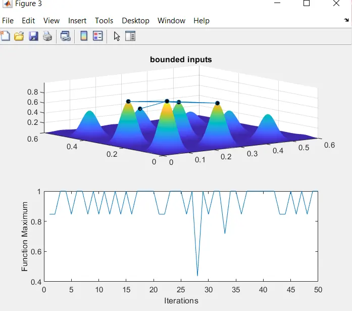
figure(3)
subplot(2,1,1)
surfc(x,y,-f)
hold on
shading interp
plot3(xopt,yopt,-fopt,'marker','o','markersize',5,'markerfacecolor','k')
title('bounded inputs');
subplot(2,1,2)
plot(-fopt)
xlabel('Iterations');
ylabel('Function Maximum');
studytime2 = toc

%study 3 - Bounded points ; incresing GA inputs
options = optimoptions('ga')
options = optimoptions(options, 'populationsize',180)

tic
for i = 1:n
    [inputs , fopt(i)] = ga(@stalagmite,2,[],[],[],[],[0;0],[0.6;0.6],[],[],options)
    xopt = inputs(1);
    yopt = inputs(2);
end

%plotting
figure(4)
subplot(2,1,1)
hold on
surfc(x,y,-f)
shading interp
plot3(xopt,yopt,-fopt,'marker','o','markersize',8,'markerfacecolor','r')
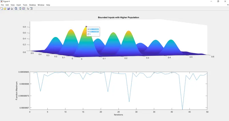
title('Bounded Inputs with Higher Population')
subplot(2,1,2)
plot(-fopt)
xlabel('Iterations')
ylabel('Function Maximum')
Studytime3 = toc

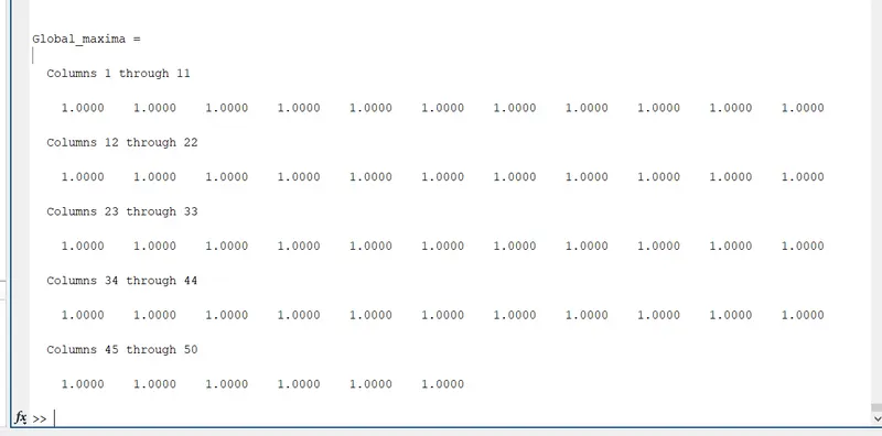
Global_maxima = -fopt
OUTPUT :
GENERAL STALAGMITE:
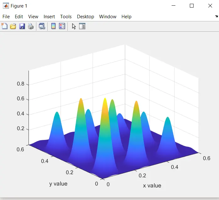
STUDY 1 - FOR UNBOUNDED INPUTS:
studytime1 = 2.4325
Here we fix the no of iterations(n) as 50 and run it for random samples.
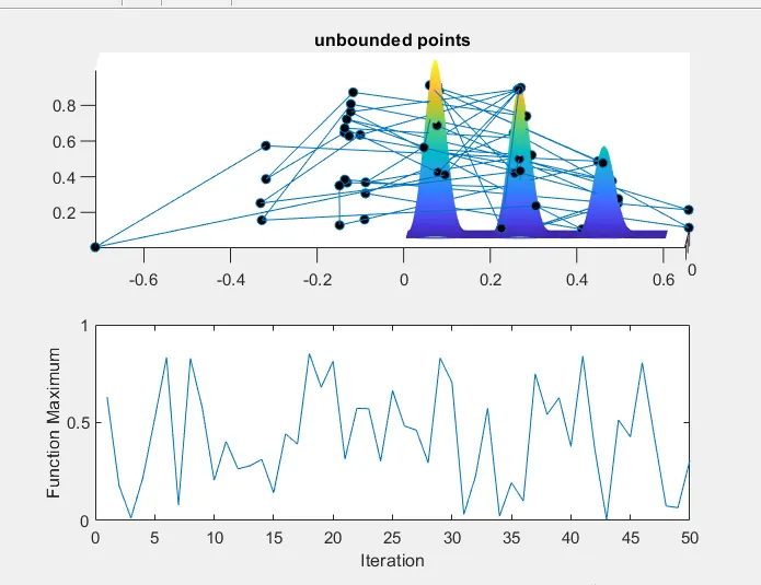
STUDY 2 - FOR BOUNDED INPUTS:
studytime2 = 3.4247
Here we fix the upper boundary and lower boundary and run the samples to find global maxima.
STUDY 3 - Optimization , increasing the population size (bounded inputs)
Studytime3 = 8.1971
We optimize the code and increase the population size to get global maxima.
ERROR FACED:
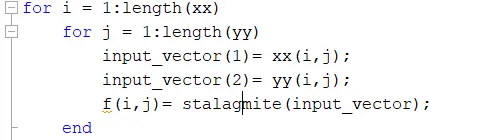
Type error - Gave a wrong function name
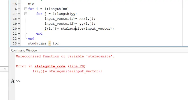
Correction:
CONCLUSION:
Thus, the global maxima have been found.
Generic algorithm(ga) is used to find optimized value for global maxima of stalagmite function.
REFERENCES:
https://in.mathworks.com/discovery/genetic-algorithm.html
https://in.mathworks.com/help/gads/how-the-genetic-algorithm-works.html
https://in.mathworks.com/help/gads/ga.html#bs08mt7-1_sep_budidgf-nvars