Week 3 - Solving second order ODEs

AIM:

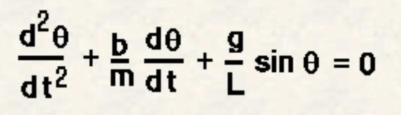
To write a program that solves the following ODE. This ODE represents the equation of motion of a simple pendulum with damping.

ODE EQUATION:

Here,

g = gravity in m/s2,

L = length of the pendulum in m,

m = mass of the ball in kg,

b=damping coefficient.

INPUTS:

L=1 metre,

m=1 kg,

b=0.05.

g=9.81 m/s2

FUNCTION CODE:

function [dtheta_dt] = ode_func(t,theta,b,g,l,m)
   theta1 = theta(1)
   theta2 = theta(2)
   dtheta1_dt=theta2;
   dtheta2_dt= -(b/m)*theta2 - (g/l)*sin(theta1);
   dtheta_dt = [dtheta1_dt ; dtheta2_dt];
end

CODE with step by step explanation:

close all
clear all
clc

%Inputs
b=0.05;
g=9.81;
l= 1;
m=1;

%Initial condition 
theta_0 = [0;3];

%time points
t_span = linspace(0,20,600);
%ode45 - inbuilt function that accepts only 1st oder equation ; @-
%anonyomous; (t,theta)- main inputs to be found, ode_func - calling a
%function; t_span and theta_0 are intial conditions
[t,results]= ode45(@(t,theta) ode_func(t,theta,b,g,l,m),t_span,theta_0);
figure(1)
plot(t,results(:,1))
hold on 
plot(t,results(:,2))
ylabel('Plot')
xlabel('Time')
legend('Angular displacement','Angular velocity')

ct=1;

for j = 1:length(results(:,1))
      x0 = 0;
      y0 = 0;
      x1 = l*sin(results(j,1));
      y1 = -l*cos(results(j,1));
      figure(2)
      plot([-.5,.5],[0,0],'-','linewidth',2,'color','k')
      hold on
      plot([x0 x1],[y0 y1],'color','b');
      hold on
      plot(x1,y1, 'marker','.','markersize',30,'color','r')
      axis([-2 2 -2 2])
      M(ct) = getframe(gcf);
      ct=ct+1;
      hold off
end

%creating an animation 
movie(M)
videofile=VideoWriter('solvingode.avi','Uncompressed AVI');
open(videofile)
writeVideo(videofile,M)
close(videofile)

1. close all - to close the plots and animation
clear all - to clear the workspace
clc - to clear command window

2. b=0.05;
g=9.81;
l= 1;
m=1;

These are the Inputs given.

3.theta_0 = [0;3]; - Inital condition where angular displacement = 0 and angular velocity = 3

4. t_span = linspace(0,20,600); - time points are taken for t = 0-20 secs and run for 600 intervals

5.[t,results]= ode45(@(t,theta) ode_func(t,theta,b,g,l,m),t_span,theta_0);

here, ode45 - inbuilt function that accepts only 1st oder equation ; @-anonyomous; (t,theta)- main inputs to be found, ode_func - calling a function; t_span and theta_0 are intial conditions.

6.figure(1)
plot(t,results(:,1))
hold on
plot(t,results(:,2))
ylabel('Plot')
xlabel('Time')
legend('Angular displacement','Angular velocity')

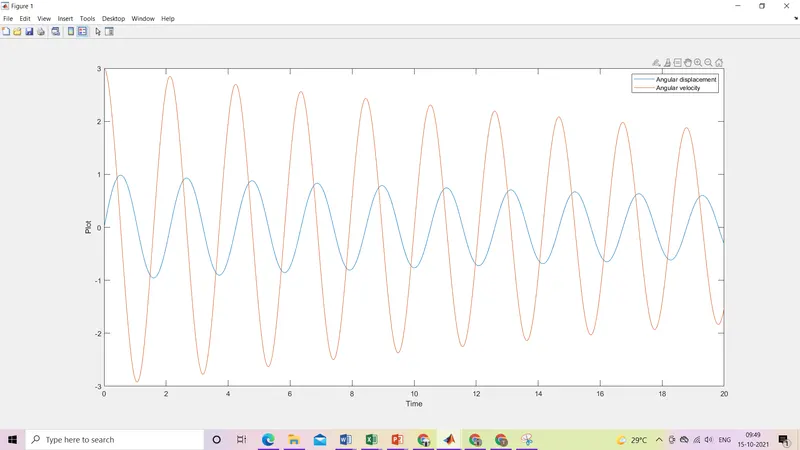
here, we plot time vs angular displacement and velocity

7.

ct=1;

for j = 1:length(results(:,1))
x0 = 0;
y0 = 0;
x1 = l*sin(results(j,1));
y1 = -l*cos(results(j,1));
figure(2)
plot([-.5,.5],[0,0],'-','linewidth',2,'color','k')
hold on
plot([x0 x1],[y0 y1],'color','b');
hold on
plot(x1,y1, 'marker','.','markersize',30,'color','r')
axis([-2 2 -2 2])
M(ct) = getframe(gcf);
ct=ct+1;
hold off
end

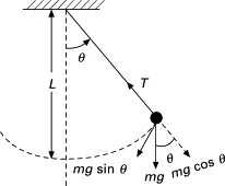here , x1 = l*sin(theta) and y = - l*cos(theta)

for loop is used to run till length of displacement values to observe the motion of pendulum

x0 and y0 values are set as zero from the above diagram.

then we create a plot to create a horizontal line

using hold on to use same plot

then we plot the Line for points (x0,y0) and (x1,y1)

then again we use hold on to use same plot

then we plot the Bob for the pendulum using marker command

get the frame using get frame command

and incrrament ct

then we use hold off and end the for loop

8.

movie(M)
videofile=VideoWriter('solvingode.avi','Uncompressed AVI');
open(videofile)
writeVideo(videofile,M)
close(videofile)

here, we create an animation by joining each frame, defining the videofile, opening the videofile , writing it and closing the videofile.

PLOT:

ERRORS :

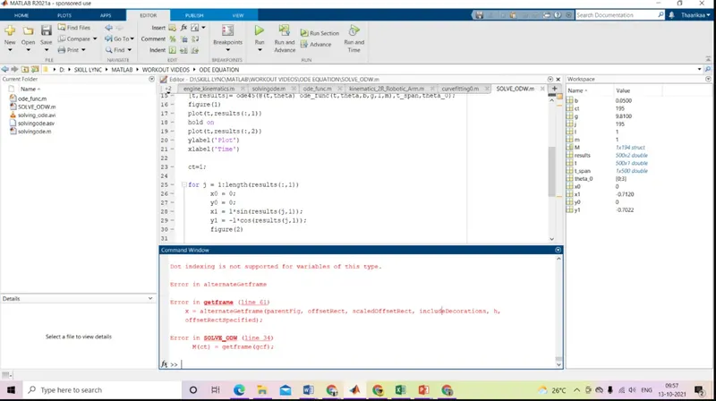
1. I closed the animation plot before it had run completely. So that I didn't get my animation as all frames weren't collected.

Correction: to Let the program run completely.

MOTION OF SIMPLE PENDULUM:

https://youtu.be/f7ntxJDVHsw

INFERENCE:

ODE45 is an inbuilt Matlab function that can solve any first-order equation.

We observe that when the damping coefficient is set low, there is the free movement of the pendulum. If we increase the damping coefficient, there will be resistance in movement.