Week 4.1 - Genetic Algorithm

AIM:

To write the code to calculate the global maxima of the stalagmite function and to explain the syntax for genetic algoritham(ga) in MATLAB.

OBJECTIVE:

• To write a code in MATLAB to optimize the stalagmite function and find global maxima of the function.
• To explain the concept of genetic algoritham and the syntax for ga in MATLAB.
• To plot the graph of all three studies and also for global maxima.

THEORY :

CODE:

x = linspace(0,0.6,150);
y = linspace(0,0.6,150);
num_cases=50;

%creating 2dimiensional grid
[xx, yy] = meshgrid(x,y);

% evaluating the stalagmite function

for i = 1:length(xx)
    for j = 1:length(yy)
        input_vector(1)= xx(i,j);
        input_vector(2)= yy(i,j);
        f(i,j) = stalagmite(input_vector);
    end

end

surf(xx, yy, f)
shading interp

xlabel('x value')
ylabel('y value')
[x_output ,fval] = ga(@stalagmite,2);

%study_1  statistical behaviour

tic
for i = 1:num_cases
[inputs,Fopt(i)] = ga(@stalagmite,2);
xopt(i) = inputs(1);
yopt(i) = inputs(2);
end

study_time_1 = toc;

%plotting 
figure(1)
subplot(2,1,1);
hold on
surfc(xx,yy,f);
shading interp;

ylabel('Y data');
xlabel('X data');
plot3(xopt,yopt,Fopt,'marker','o','markersize',5,'markerfacecolor','y')
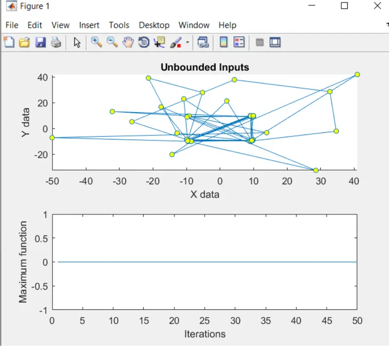
title('Unbounded Inputs')
subplot(2,1,2)
plot(Fopt)
xlabel('Iterations')
ylabel('Maximum function')


%study_2 bounding the values

tic
for i = 1:num_cases
[inputs,Fopt(i)] = ga(@stalagmite,2,[],[],[],[],[0;0],[1;1]);
xopt(i) = inputs(1);
yopt(i) = inputs(2);
end
study_time_2 = toc;


figure(2)
subplot(2,1,1)
hold on
surfc(xx,yy,f)
shading interp
xlabel('X data')
ylabel('Y data')
plot3(xopt,yopt,Fopt,'marker','o','markersize',5,'markerfacecolor','r');
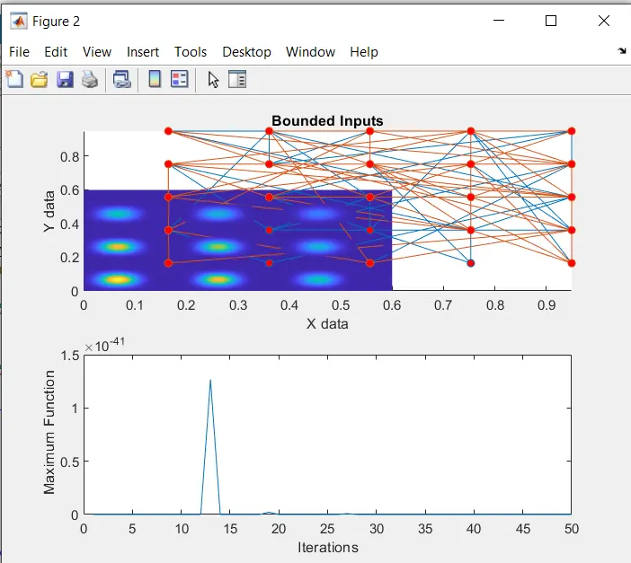
title('Bounded Inputs')
subplot(2,1,2)
plot(Fopt)
xlabel('Iterations')
ylabel(' Maximum Function')



%study_3 bounding the values and increasing population size 

options = optimoptions('ga');
options = optimoptions(options,'populationsize',300);
tic
for i = 1:num_cases
[inputs,Fopt(i)] = ga(@stalagmite,2,[],[],[],[],[0;0],[1;1],[],[],options);
xopt(i) = inputs(1);
yopt(i) = inputs(2);
end

study_time_3 = toc;

figure(3)
subplot(2,1,1)
hold on
surfc(xx,yy,f)
shading interp
xlabel('X data')
ylabel('Y data')
plot3(xopt, yopt,Fopt,'marker','o','markersize',5,'markerfacecolor','g');
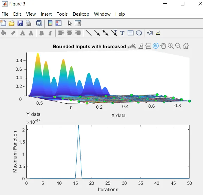
title('Bounded Inputs with Increased population size');
subplot(2,1,2)
plot(Fopt)
xlabel('Iterations');
ylabel('Maximum Function');

Firstly we initialise the values of x and y taking 150 values between the interval 0 and 0.6 Then we consider no of iterations num_spaces=50. Since we need to plot a 3D surface plot we take the 2d array of x and y using meshgrid command and store them in input_vector array ,so that it can be used as an argument to call the function stalagmite we create another fuction file for the stalagmite function. here we take the ouput as -f since ga only minimises a given function.so if -f is considered it automatically gives us the maxima.

First case study-

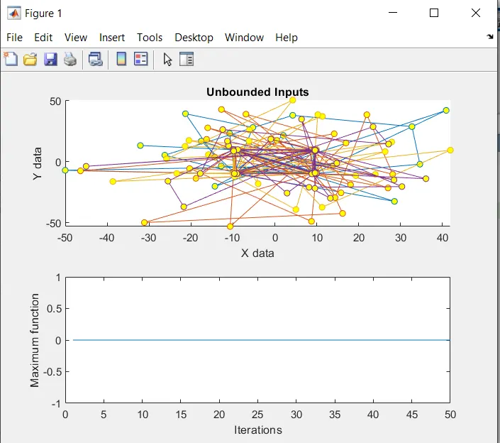
We first take no of iterations = num_spaces and we use the genetic algorithm function to caluclate the maxima of the function. Then we store the outputs into results which contain maximas and fopt which contain the value at which the maxima is obtained. Here the ga is initiated with random population. Then we store the results into xopt, yopt.now we need to plot the surface of x,y,-f to get the 3D plot.We use the plot3 command to make a plot of xopt,yopt and -fopt to plot the optimum maximas. Also let us plot the fopt functio so that we can visualise the optimum values at each iteration. To get the time taken to complete cycle we used the tic toc commands to record the time.

Second case study:

We set the boundary conditions in this part. Let us specify the lower and upper bounds of x and y in this case,the ga is initiated with random population only. Then we store the results into xopt, yopt.now we need to plot the surface of x,y,-f to get the 3D plot.We use the plot3 command to make a plot of xopt,yopt and -fopt to plot the optimum maximas.Also let us plot the fopt functio so that we can visualise the optimum values at each iteration. To get the time taken to complete cycle we used the tic toc commands to record the time.

Third case study:

In this case let us increase our initial population to 300. We store the results into xopt, yopt.now we need to plot the surface of x,y,-f to get the 3D plot.We use the plot3 command to make a plot of xopt,yopt and -fopt to plot the optimum maximas.Also let us plot the fopt functio so that we can visualise the optimum values at each iteration. To get the time taken to complete cycle we used the tic toc commands to record the time.

FUNCTION CODE:

function [f]=stalagmitefunction(input_vector)

x=input_vector(1);
y=input_vector(2);
f1=(sin(5.1*pi*x+0.5))^6;
f2=(sin(5.1*pi*y+0.5))^6;
f3=exp(-4*log(2)*(x-0.0667)^2/0.64);
f4=exp(-4*log(2)*(y-0.0667)^2/0.64);

f=(f1*f2*f3*f4);
end

OUTPUTS:

ERRORS:

I did not face any errors other than the one asking me to install General Algorithm Toolbox.