Week 4.1 - Genetic Algorithm

Stalagmite function

Aim:

To write a program to optimize the stalagmite function and find the global maxima of the function.

Theory:

Genetic algorithim is a search based optimization technique based on the principles of genetics and natural selection.gentic algorithim is generally used to solve optimization problems.

Optimization:

It is like a feedback loop where the input values will be changed based upon the required output values .the input values will be changed upon each iteration to get the desired output value.

Principle of genetic algorithm:

• For a given problem statement ,we will have a population of possible solutions.
• They undergo recombination and mutattion to produce the next set of outputs(the children).
• The children are pooled together and they are numbered.
• Here with the help of fitness score I.e a filteration score, fitter individuals are selecte.
• These selected individuals are then allowed to reproduce randomly,which results in a crossover of the species(solutions).
• The crossover of the fitter generation can result in both positvely and negatively mutated children. This mutation is caused to maintain the diversity in the population.

Natural selection:

The factors that constitute the process of natural selection are

• Initial population
• Fitness score
• Crossover
• Mutation

Final note : the fitness score acts as a filter not as a stopping criteria. The stopping criteria happens when there is no mutation and the population comes to a stand still.

The stopping criteria:

In genetic algorithm, the stopping criteria depends upon three things

• the input matrix
• The number of iterations.
• Final output of the calling function.(in this program)
• Limits if its specified

  Syntax for genetic algorithm:

  x = ga(fun,nvars)
  x = ga(fun,nvars,A,b)
  x = ga(fun,nvars,A,b,Aeq,beq)
  x = ga(fun,nvars,A,b,Aeq,beq,lb,ub)
  x = ga(fun,nvars,A,b,Aeq,beq,lb,ub,nonlcon)
  x = ga(fun,nvars,A,b,Aeq,beq,lb,ub,nonlcon,options)
  x = ga(fun,nvars,A,b,[],[],lb,ub,nonlcon,IntCon)
  x = ga(fun,nvars,A,b,[],[],lb,ub,nonlcon,IntCon,options)
  x = ga(problem)
  [x,fval] = ga(___)
  [x,fval,exitflag,output] = ga(___)
  [x,fval,exitflag,output,population,scores] = ga(___)​

  Program:
  clear all
  close all
  clc
   
  %input$
  x = linspace(0,0.6,150);
  y = linspace(0,0.6,150);
  num_spaces = 50;
   
  %forming 2d array%
  [xx,yy] = meshgrid(x,y);
  for i = 1: length(xx)
      for j = 1: length(yy)
          input_vector(1) = xx(i,j);
          input_vector(2) = yy(i,j);
          f(i,j)=stalagmite(input_vector);
      end
  end
  %study 1- unbounded%
  tic
  for i = 1:num_spaces
      [results,fopt(i)]= ga(@stalagmite,2);
      xopt(i) = results(1);
      yopt(i) = results(2);
  end
  study_time=toc
  figure(1)
  subplot(2,1,1)
  surf(x,y,-f)
  shading interp
  hold on
  plot3(xopt,yopt,-fopt,'marker','o'); 
  subplot(2,1,2)
  plot(-fopt)
  xlabel('iteration')
  ylabel('function maximum')
   
  %study2-unbounded%
  tic
  for i=1:num_spaces
      [results,fopt(i)]= ga(@stalagmite,2,[],[],[],[],[0;0],[0.6;0.6]);
      xopt(i)=results(1);
      yopt(i)=results(2);
  end
  study_time2=toc
  figure(2)
  subplot(2,1,1)
  surf(x,y,-f)
  shading interp
  hold on
  plot3(xopt,yopt,-fopt,'marker','o')
  subplot(2,1,2)
  plot(-fopt)
  xlabel('iteration')
  ylabel('function maximum')
   
  %study-3 increased initial population%
  options=optimoptions('ga');
  options=optimoptions(options,'populationsize',700);
  tic
  for i= 1:100
      [results,fopt(i)]=ga(@stalagmite,2,[],[],[],[],[0;0],[0.1;0.1],[],[],options);
      xopt(i)=results(1);
      yopt(i)= results(2);
  end
  study_time3=toc 
  figure(3)
  subplot(2,1,1)
  surf(x,y,-f)
  shading interp
  hold on
  plot3(xopt,yopt,-fopt,'marker','o')
  subplot(2,1,2)
  plot(-fopt)
  xlabel('iteration')
  ylabel('function maximum')
  
  Stalgmite function.
  function A = stalagmite (input_vector)
  x= input_vector(1);
  y= input_vector(2);
  f1= (sin(5.1*pi*x+0.5)).^6;
  f2= exp((-4*log(2)*((x-0.0667).^2))/0.64);
  f3=(sin(5.1*pi*y+0.5)).^6;
  f4= exp((-4*log(2)*((y-0.0667).^2))/0.64);
  A=-(f1*f2*f3*f4);
  end​

  Program code explanation:

  • First we intialise the inputs, I.e declare the inputs.
  • Now the values of x,y have been declared with 150 variables in-between 0-0.6.
  • Meshgrid command was used to convert the inputs into a 2-D array,after converting now we store this variable into 2 inputs basically we declare the inputs.. convert it into 2-d array and store it into 2 separate variables so that it can be used as a matrix. Thats the key.
  • Now we create a separate function for stalagmite,now we know the ga corner downs the result to the most least value. So therefore we use -f to get the global maxima

  .

  • %study-1%- unbounded
  • Here we intitate the iteration using for loop, next we use the surface command to visualize the outputs of (x,y,-f).
  • Tic toc command is used to note the time taken for iteration to get completed.
  • Plot3 command is used to plot the optimum values of x,y and f ..then this command is used to plot the global maxima.
  • %study-2%-bounded
  • Here we specify the lower and upper bound of the x.y and the program is simulated.
  • %study-3%-bounded with intial population
  • The intial population of the program is set to be 700, and the same code is executed.

  The timings of each study is given as

  Study1- 5.3712

  Study2-5.0332

  Study3-78.1049

  Errors faced while doing the program:

  1. Used . while declaring the inputs [results.fopt(I)]
  2. did not declare f(I,j)=stalagmite(input_vector) during the intial iteration for the for loop.
  3. In stalagmite function code was using the value (x-0.6667) instead of (x-0.0667).
  4. While declaring 2-d arrays we used
     [xx, yy]=meshgrid[x,y]
     for I= 1:length(x);
     for j= 1: lenght(y)
     
     Instead of
     for I = 1:length(xx)
     for j = 1:length(yy)

Output:

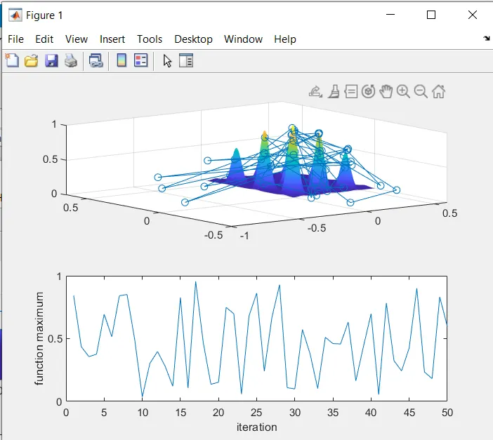
output1

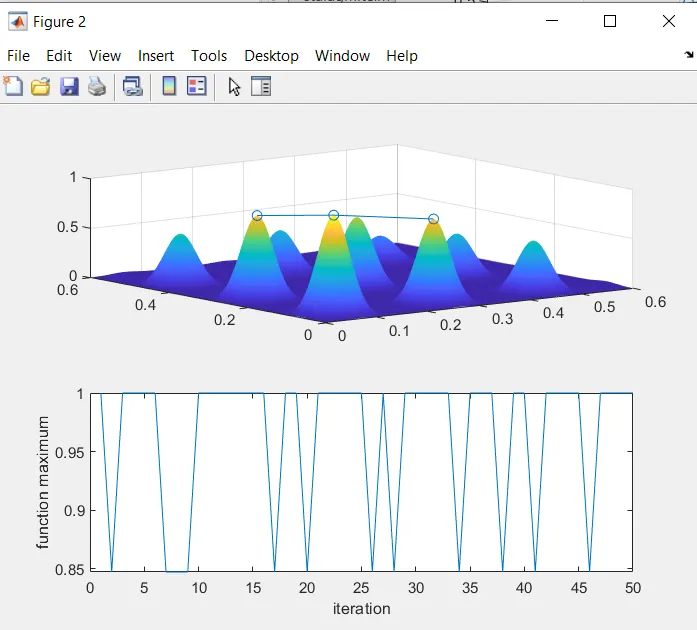
Output2

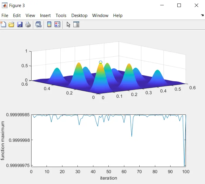
Output3