Week 4.1 - Genetic Algorithm

AIM

To write a code in matlab to optimise the stalagmite function and find the global maxima of the function and also explain the syntax for ga in matlab.

Objective

• Write a matlab code to optmise the stlagmite function
• Explain the concept of genetic algoritham and its syntax in matlab
• Plot the graphs for all the three studies and for F maximum vereses number of iterations

Theory

Stalagmites

Stalagmites are convex deposits that grow upward, commonly fed by an overhanging stalactite, and show flat, rounded or slightly hollow tops, but not a central canal. Calcite and aragonite stalagmites form through degassing of a saturated thin film of fluid (about 0.1-mm thick), which slowly moves down from the stalagmite tip to its flanks. The morphology of stalagmites is mostly determined by the drip rate, and in particular by the interannual variability of the drip rate and by the distance from the tip of the feeding stalactite.

Genetic algoritham

Genetic algorithms are randomized search algorithms that have been developed in an effort to imitate the mechanics of natural selection and natural genetics. Genetic algorithms operate on string structures, like biological structures, which are evolving in time according to the rule of survival of the fittest by using a randomized yet structured information exchange. Thus, in every generation, a new set of strings is created, using parts of the fittest members of the old set. The main characteristics of a genetic algorithm are as follows:

(1).The genetic algorithm works with a coding of the parameter set, not the parameters themselves.

(2).The genetic algorithm initiates its search from a population of points, not a single point.

(3).The genetic algorithm uses payoff information, not derivatives.

(4).The genetic algorithm uses probabilistic transition rules, not deterministic ones.

Limitations

1.GA implementation is still an art

2.GA requires les information about the problem but designing an objective function and getting the representation and operators right can be difficult.

3.GA is computationally time consuming.

Mathematical equation

fs=-f1x*f2x*f1y*f2y

where, f1x=(sin(5.1*pi*x+.5))^6

 f1y=(sin(5.1*pi*y+.5))^6

f2x=exp[-4ln(2)((x-.667)^2)/.64]

f2x=exp[-4ln(2)((y-.667)^2)/.64]

 Stalagmite function programme for mathematical equation

function [fs]=stalagmite(input_vector)
x=input_vector(1);
y=input_vector(2);
 f1x=(sin(5.1*pi*x+.5))^6;
 f1y=(sin(5.1*pi*y+.5))^6;
 f2x=exp(-4*log(2)*((x-.0667)^2)/.64);
 f2y=exp(-4*log(2)*((y-.0667)^2)/.64);
 fs=-f1x*f2x*f1y*f2y;
end

programme for ploting the global maxima

clear all 
close all
clc
x=linspace(0,0.6,150);
y=linspace(0,0.6,150);
num_cases=50
[xx,yy]=meshgrid(x,y);

% evaluating the slalagmite function
for i=1:length(xx)
    for j=1:length(yy)
        input_vector(1)=xx(i,j);
        input_vector(2)=yy(i,j);
        f(i,j)=stalagmite(input_vector);
        
    end
end
surfc(xx,yy,-f)
xlabel('x value')
ylabel('y value')
% shading interp
[inputs,fval]=ga(@stalagmite,2)

programme for ploting the global minima and finding the minimum function used by 3 study cases

study1

clear all 
close all
clc
x=linspace(0,0.6,150);
y=linspace(0,0.6,150);
num_cases=50
[xx,yy]=meshgrid(x,y);

% evaluating the slalagmite function
for i=1:length(xx)
    for j=1:length(yy)
        input_vector(1)=xx(i,j);
        input_vector(2)=yy(i,j);
        f(i,j)=stalagmite(input_vector);
        
    end
end
for i=1:num_cases
    [inputs,fopt(i)]=ga(@stalagmite,2);
    xopt(i)=inputs(1);
    yopt(i)=inputs(2);
end
figure(1)
subplot(2,1,1);
hold on 
surfc(x,y,f)
shading interp
plot3(xopt,yopt,fopt,'marker','o','markersize',5,'markerfacecolor','r');
title('unbounded inputs');
subplot(2,1,2)
plot(fopt)
xlabel('iterations')
ylabel('functions minimmum')

study2

clear all 
close all
clc
x=linspace(0,0.6,150);
y=linspace(0,0.6,150);
num_cases=50
[xx,yy]=meshgrid(x,y);

% evaluating the slalagmite function
for i=1:length(xx)
    for j=1:length(yy)
        input_vector(1)=xx(i,j);
        input_vector(2)=yy(i,j);
        f(i,j)=stalagmite(input_vector);
        
    end
end
% study1-statistical beaviour
tic
for i=1:num_cases
    [inputs,fopt(i)]=ga(@stalagmite,2,[],[],[],[],[0;0],[1;1]);
    xopt(i)=inputs(1);
    yopt(i)=inputs(2);
end
study2_time=toc
figure(2)
subplot(2,1,1);
hold on 
surfc(x,y,f)
% shading interp
plot3(xopt,yopt,fopt,'marker','o','markersize',5,'markerfacecolor','r');
title('unbounded inputs');
subplot(2,1,2)
plot(fopt)
xlabel('iterations')
ylabel('functions minimum')

study3

clear all 
close all
clc
x=linspace(0,0.6,150);
y=linspace(0,0.6,150);
num_cases=50
[xx,yy]=meshgrid(x,y);

% evaluating the slalagmite function
for i=1:length(xx)
    for j=1:length(yy)
        input_vector(1)=xx(i,j);
        input_vector(2)=yy(i,j);
        f(i,j)=stalagmite(input_vector);
        
    end
end
% study3-statistical beaviour
options=optimoptions('ga');
options=optimoptions(options,'populationsize',170);
tic
for i=1:num_cases
    [inputs,fopt(i)]=ga(@stalagmite,2,[],[],[],[],[0;0],[.1;.1],[],[],options);
    xopt(i)=inputs(1);
    yopt(i)=inputs(2);
end
study3_time=toc
figure(3)
subplot(2,1,1);
hold on 
surfc(x,y,f)
% shading interp
plot3(xopt,yopt,fopt,'marker','o','markersize',5,'markerfacecolor','r');
title('unbounded inputs');
subplot(2,1,2)
plot(fopt)
xlabel('iterations')
ylabel('functions minimum')

output

for global maxima

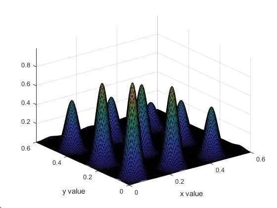
For finding the global minimum function by ga

study1 output plot

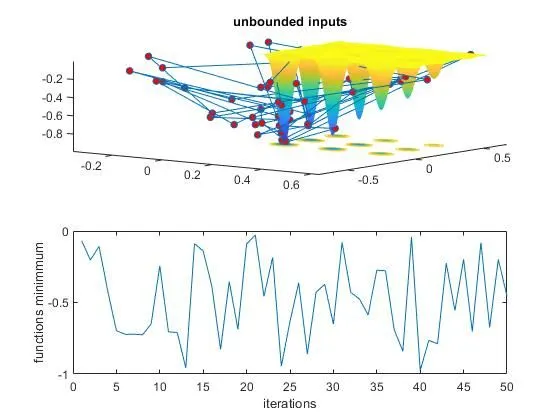
Study2 output plot

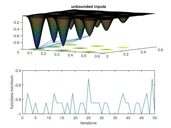
Study3 output plot

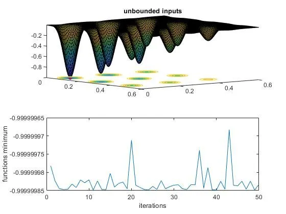
Results

• Code for global maxima and stalagmite function done
• The concept study and explanation of genetic algoritham is done
• The graphs of global axima and the three case studies are plotted

References

https://www.sciencedirect.com/topics/engineering/genetic-algorithm

https://en.wikipedia.org/wiki/Genetic_algorithm