Week 4.1 - Genetic Algorithm

Genetic algorithem

AIM : To calculate next population values in future by reference of present population by using global optimaization in mat lab

Theory :

A genetic algorithm (GA) is a method for solving both constrained and unconstrained optimization problems based on a natural selection process that mimics biological evolution. The algorithm repeatedly modifies a population of individual solutions. At each step, the genetic algorithm randomly selects individuals from the current population and uses them as parents to produce the children for the next generation. Over successive generations, the population "evolves" toward an optimal solution.

You can apply the genetic algorithm to solve problems that are not well suited for standard optimization algorithms, including problems in which the objective function is discontinuous, nondifferentiable, stochastic, or highly nonlinear.

CODE :

% stalgamite
close all
clear all
clc
 % defining search space
 x = linspace(0,0.7,155);
 y = linspace(0,0.7,155);
 [x,y]= meshgrid(x,y);
 num_case=50;
 
 for i=1:length(x)
     for j=1:length(y)
         input_vector(1)=x(i,j);
         input_vector(2)=y(i,j);
         f(i,j)= stalagmite(input_vector);
     end
 end
 
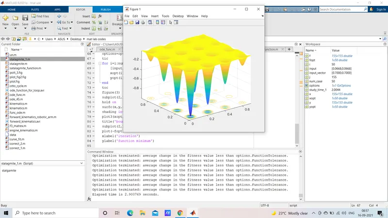
 surfc(x,y,f);
 shading interp
 
 
 %study-1 statistical behavior
 tic
 for i=1:num_case
     [input,fopt(i)]=ga(@stalagmite,2);
     xopt(i)=input(1);
     yopt(i)=input(2);
 end
 
 study_time_1=toc
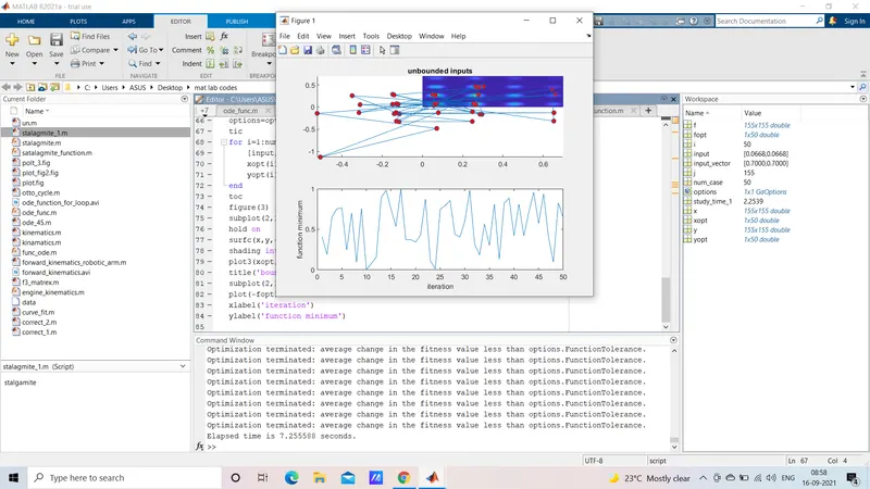
 figure(1)
 subplot(2,1,1);
 hold on
 surfc(x,y,-f);
 shading interp
 plot3(xopt,yopt,-fopt,'marker','o','markersize',6,'markerfacecolor','r')
 title('unbounded inputs')
 subplot(2,1,2)
 plot(-fopt)
 xlabel('iteration')
 ylabel('function minimum')
 
 %study-2-statistical behavoir with upper and lower bounds
 tic
 for i=1:num_case
     [input,fopt(i)]=ga(@stalagmite,2,[],[],[],[],[0;0],[1;1]);
         xopt(i)=input(1);
         yopt(i)=input(2);
 end
toc
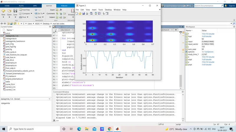
figure(2)
subplot(2,1,1)
hold on
surfc(x,y,-f)
shading interp
plot3(xopt,yopt,-fopt,'marker','o','markersize',6,'markerfacecolor','r');
subplot(2,1,2)
plot(-fopt)
xlabel('iteration')
ylabel('function minimum')


%study 3 increasing the ga iterations
options = optimoptions('ga');
options=optimoptions(options,'populationsize',200);
tic
for i=1:num_case
    [input,fopt(i)]=ga(@stalagmite,2,[],[],[],[],[0;0],[1;1],[],[],options);
    xopt(i)=input(1);
    yopt(i)=input(2);
end
toc
figure(3)
subplot(2,1,1)
hold on 
surfc(x,y,-f)
shading interp
plot3(xopt,yopt,-fopt,'marker','o','markersize',6,'markerfacecolor','r');
title('bounded input')
subplot(2,1,2)
plot(-fopt)
xlabel('iteration')
ylabel('function minimum')



function f=stalagmite(input_vector)
x=input_vector(1);
y=input_vector(2);
f1=[sin(5.1*pi*x+0.5)].^6;
f2=[sin(5.1*pi*y+0.5)].^6;
f3=exp(-4*log(2)*[x-0.0667].^2/0.64);
f4=exp(-4*log(2)*[y-0.0667].^2/0.64);
f=-(f1*f2*f3*f4);
end

RESULT :