Week 4.1 - Genetic Algorithm
Aim:To calculate the global maxima of stalagmite function using MATLAB.
Introduction:
Genetic Algorithm consists a class of probabilistic optimization algorithms. GENETIC ALGORITHM MATLAB tool is used in computing to find approximate solutions to optimization and search problems. Set of possible solutions are randomly generated to a problem, each as fixed length character string. Keep best solution to generate new possible solutions.
What are Genetic Algorithms?
Nature has always been a great source of inspiration to all mankind. Genetic Algorithms (GAs) are search based algorithms based on the concepts of natural selection and genetics. GAs are a subset of a much larger branch of computation known as Evolutionary Computation.
GAs were developed by John Holland and his students and colleagues at the University of Michigan, most notably David E. Goldberg and has since been tried on various optimization problems with a high degree of success.
In GAs, we have a pool or a population of possible solutions to the given problem. These solutions then undergo recombination and mutation (like in natural genetics), producing new children, and the process is repeated over various generations. Each individual (or candidate solution) is assigned a fitness value (based on its objective function value) and the fitter individuals are given a higher chance to mate and yield more “fitter” individuals. This is in line with the Darwinian Theory of “Survival of the Fittest”.
In this way we keep “evolving” better individuals or solutions over generations, till we reach a stopping criterion.
Genetic Algorithms are sufficiently randomized in nature, but they perform much better than random local search (in which we just try various random solutions, keeping track of the best so far), as they exploit historical information as well.
Advantages of GAs
GAs have various advantages which have made them immensely popular. These include −
-
Does not require any derivative information (which may not be available for many real-world problems).
-
Is faster and more efficient as compared to the traditional methods.
-
Has very good parallel capabilities.
-
Optimizes both continuous and discrete functions and also multi-objective problems.
-
Provides a list of “good” solutions and not just a single solution.
-
Always gets an answer to the problem, which gets better over the time.
-
Useful when the search space is very large and there are a large number of parameters involved.
Limitations of GAs
Like any technique, GAs also suffer from a few limitations. These include −
-
GAs are not suited for all problems, especially problems which are simple and for which derivative information is available.
-
Fitness value is calculated repeatedly which might be computationally expensive for some problems.
-
Being stochastic, there are no guarantees on the optimality or the quality of the solution.
-
If not implemented properly, the GA may not converge to the optimal solution.
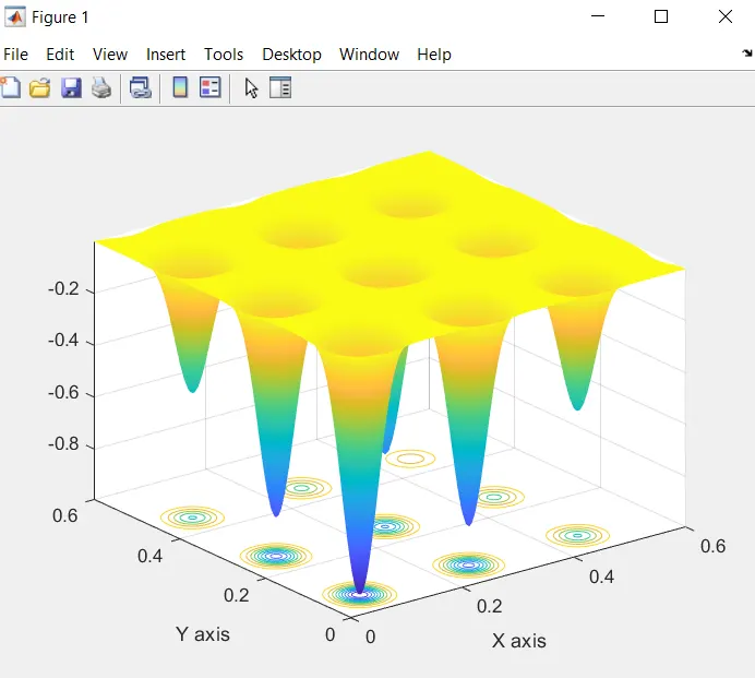
stalagmite function :stalagmite function is the mathematical model actually help us to gain local maxima and minimas . A stalagmite is the type of rock formation that rises from the floor of the cave due t the accumulation of the material deposited on the floor from ceiling drippings . stalagmite may be composed of lava ,minerals and sand etc. 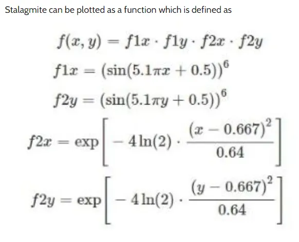
Genetic algorithm syntax: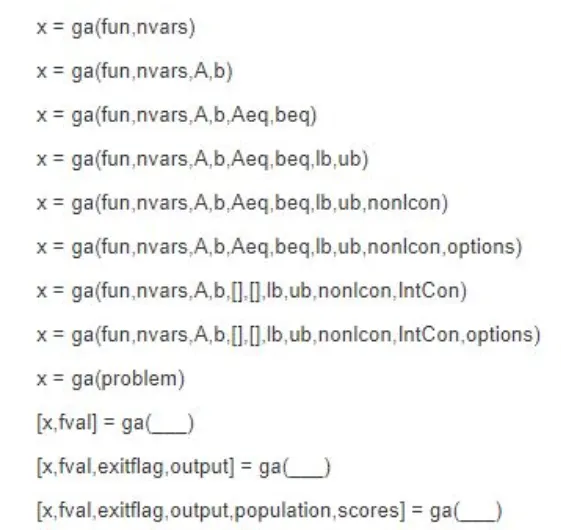
Objective:To optmize the stalagmite function.
To determine the global maxima using genetic algorithm.
Code:
stalagmite function code:
function f = stalagmite1(input_vector)

x = input_vector(1);
y = input_vector(2);

f1 = [sin(5.1*pi*x+0.5)].^6;
f2 = [sin(5.1*pi*y+0.5)].^6;
f3 = exp(-4*log(2)*[x-0.0667].^2/0.64);
f4 = exp(-4*log(2)*[y-0.0667].^2/0.64);

f = -(f1*f2*f3*f4);
end
Genetic algorithm code:
% Defining our search space
x=linspace(0,0.6,150);
y=linspace(0,0.6,150);

num_cases=50; % To run the ga 50 times

[X,Y]=meshgrid(x,y)

% Evaluating the stalagmite function
for i=1:length(X)
    for j=1:length(Y)
        input_vector(1)= X(i,j);
        input_vector(2)= Y(i,j);
        f(i,j)=stalagmite1(input_vector);
% stalagmite function takes in the data given inside parantheses and calculates f
    end
end
surfc(X,Y,f);
xlabel('X axis')
ylabel('Y axis')
shading interp

tic
% Study 1 - Unbounded Condition
for i=1:num_cases
    [inputs,fopt(i)]=ga(@stalagmite1,2);

    % ga is an in-built function
    % @ defines what function to minimise
    % ga always minimises a function
    % 2 denotes the no. of variables in the function, here it is x and y

    xopt(i)=inputs(1);
    yopt(i)=inputs(2);
end

study1_time = toc;
% tic toc is used to measure how long it takes to study

figure(1)
subplot(2,1,1) % To have multiple plots inside the same figure window
hold on
surfc(x,y,-f)
shading interp
plot3(xopt,yopt,-fopt,'marker','o','markersize',5,'markerfacecolor','r')
title('Unbounded Inputs')
subplot(2,1,2)
plot(-fopt)
xlabel('Iterations');
ylabel('Function minimum');

tic
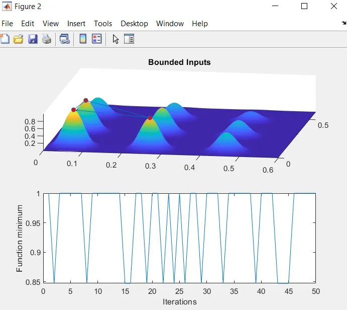
% Study 2 - Statistical behaviour - with upper and lower bounds
for i=1:num_cases
    [inputs,fopt(i)]=ga(@stalagmite1,2,[],[],[],[],[0;0],[0.6;0.6]);
    xopt(i)=inputs(1);
    yopt(i)=inputs(2);
end
study2_time=toc;

figure(2)
subplot(2,1,1)
hold on
surfc(x,y,-f)
shading interp
plot3(xopt,yopt,-fopt,'marker','o','markersize',5,'markerfacecolor','r')
title('Bounded Inputs')
subplot(2,1,2)
plot(-fopt)
xlabel('Iterations');
ylabel('Function minimum');

% Study 3 - Increasing GA Iterations
options=optimoptions('ga')
options=optimoptions(options,'PopulationSize',300);

tic
for i=1:num_cases
    [inputs,fopt(i)]=ga(@stalagmite1,2,[],[],[],[],[0;0],[0.6;0.6],[],[],options);
    xopt(i)=inputs(1);
    yopt(i)=inputs(2);
end
study3_time=toc;

figure(3)
subplot(2,1,1)
hold on
surfc(x,y,-f)
shading interp
plot3(xopt,yopt,-fopt,'marker','o','markersize',5,'markerfacecolor','r')
title('Bounded Inputs with Modified Population Size')
subplot(2,1,2)
plot(-fopt)
xlabel('Iterations');
ylabel('Function minimum');
Results and plots:
study 1 plot:
study 2 plot:
study 3 plot:
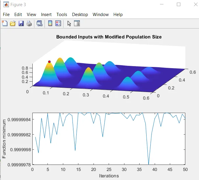
No errors face while programing
conclusion:Hence we plotted 3 studies withunbounded inputs, with upper andd lower limit and by increasing the population and have used the ga inbuilt cammand to get the global maxima.