Week 4.1 - Genetic Algorithm
%% clean all
clear all; close all;clc
%% Defining our search space
x= linspace(0,0.6,150);
y= linspace(0,0.6,150);
num_cases = 50;
% no of itration
%% Creating a 2Dimensional mesh
[xx,yy]= meshgrid(x,y);
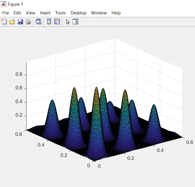
%% Evaluating the stalagmite function
for i= 1:length(xx)
for j = 1:length(yy)
input_vector(1)=xx(i,j);
input_vector(2)=yy(i,j);
input_vector=[input_vector(1),input_vector(2)];
f(i,j)=stalagmite(input_vector);
end
end
surfc(x,y,-f)
%% Study -1| Statistical Behaviour | In Unbounded condition
tic
% tic_toc command for calculating the iteration time
for i = 1:num_cases
[input,f_opt(i)]=ga(@stalagmite,2);
xopt(i) = input(1);
yopt(i) = input(2);
end
study_1_time = toc;
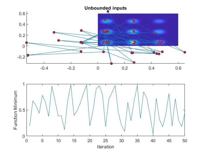
% Plotting the graph
figure(1)
subplot(2,1,1)
hold on
surfc(x,y,-f)
shading interp
plot3(xopt,yopt,-f_opt,'marker','o','markersize',5,'markerfacecolor','r')
title('Unbounded inputs')
subplot(2,1,2)
plot(-f_opt)
xlabel('Iteration')
ylabel('Function Minimum')
%% Study-2 | Stastical behaviour - with upper & lower bounds
tic
%tic_toc command for calculating the iteration time
for i= 1:num_cases
[ input,f_opt(i)] = ga(@stalagmite,2,[],[],[],[],[0;0],[1;1]);
xopt(i) = input(1);
yopt(i) = input(2);
end
study_2_time = toc;
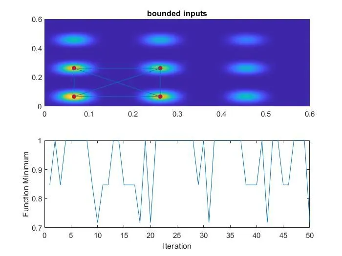
% Plotting the graph
figure(2)
subplot(2,1,1)
hold on
surfc(x,y,-f)
shading interp
plot3(xopt,yopt,-f_opt,'marker','o','markersize',5,'markerfacecolor','r')
title('bounded inputs')
subplot(2,1,2)
plot(-f_opt)
xlabel('Iteration')
ylabel('Function Minimum')
%% Study-3 | Icreasing GA Iterations
options = optimoptions ('ga');
% Calculating the optium solution for 'ga' and save in options ( varibale )
options = optimoptions(options,'populationsize',240);
% increasing the size population
tic
%tic_toc command for calculating the iteration time
for i= 1:num_cases
[ input,f_opt(i)] = ga(@stalagmite,2,[],[],[],[],[0;0],[1;1],[],[],options);
xopt(i) = input(1);
yopt(i) = input(2);
end
study_3_time = toc;
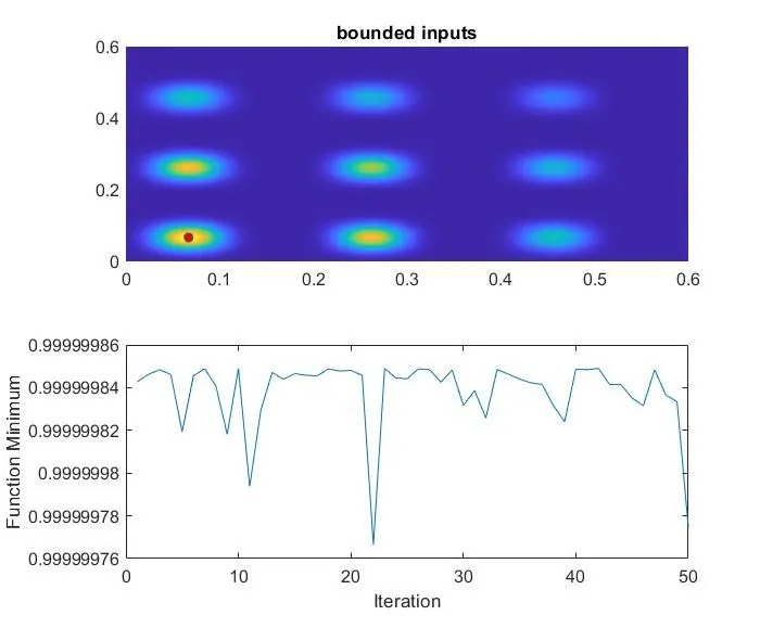
% Plotting the graph
figure(3)
subplot(2,1,1)
hold on
surfc(x,y,-f)
shading interp
plot3(xopt,yopt,-f_opt,'marker','o','markersize',5,'markerfacecolor','r')
title('bounded inputs')
subplot(2,1,2)
plot(-f_opt)
xlabel('Iteration')ylabel('Function Minimum'
unction [f] = stalagmite(input_vector)
x=input_vector(1);
y=input_vector(2);
term1 = pi*5.1*x;
term2 = pi*5.1*y;
term3 = ((x-0.0667)^2/0.64);
term4 =((y-0.0667)^2/0.64);
term5 = (-4)*log(2);
xf1 = (sin(term1+0.5)).^6;
yf1 = (sin(term2+0.5)).^6;
xf2 = exp(term5*term3);
yf2 = exp(term5*term4);
f=-(xf1*yf1*xf2*yf2);
end
AIM- To write a code in MATLAB to optimize the stalagmite function and find the
global maxima of the function.
Theory-
Genetic Algorithm (GA) is a search-based optimization technique based on the principles of Genetics & natural Selection. It is frequently used to find optimal or near optimal solutions to difficult problems which otherwise would take a lifetime to solve. It is frequently used to solve optimization problems, in research and in machine learning.
Introduction to Optimization
Optimization is an important tool in making decisions and in analysing physical systems. In mathematical terms, an optimization problem is the problem of finding the best solution from among the set of all feasible solutions.
Constructing a Model
The first step in the optimization process is constructing an appropriate model; modelling is the process of identifying and expressing in mathematical terms the objective, the variables, and the constraints of the problem.
- An objective is a quantitative measure of the performance of the system that we want to minimize or maximize. In manufacturing, we may want to maximize the profits or minimize the cost of production, whereas in fitting experimental data to a model, we may want to minimize the total deviation of the observed data from the predicted data.
- The variables or the unknowns are the components of the system for which we want to find values. In manufacturing, the variables may be the amount of each resource consumed or the time spent on each activity, whereas in data fitting, the variables would be the parameters of the model.
- The constraints are the functions that describe the relationships among the variables and that define the allowable values for the variables. In manufacturing, the amount of a resource consumed cannot exceed the available amount.
Syntax for Genetic Algorithm
x = ga(fun,nvars,A,b,Aeq,beq,lb,ub)
x = ga(fun,nvars,A,b,Aeq,beq,lb,ub,nonlcon)
x = ga(fun,nvars,A,b,Aeq,beq,lb,ub,nonlcon,options)
x = ga(fun,nvars,A,b,[],[],lb,ub,nonlcon,IntCon)
x = ga(fun,nvars,A,b,[],[],lb,ub,nonlcon,IntCon,options)
[x,fval,exitflag,output] = ga(___)
[x,fval,exitflag,output,population,scores] = ga(___)
OUTPUT OF THE CODE-