Week 4.1 - Genetic Algorithm

% in this program genetic algorithm is used to do optimization.
clear all
close all
clc
%search space
x = linspace(0, 0.6, 150);
y = linspace(0, 0.6, 150);

%2D mesh
[xx, yy] = meshgrid(x,y);

%stalagmite function evalution
g = zeros(150,150);
for i=1:length(xx)
    for j=1:length(yy)
        inp(1) = xx(i,j);
        inp(2) = yy(i,j);
        g(i,j) = stalagmite(inp);
    end
end

%Study 1- no bounds
fopt = zeros(50);
xopt = zeros(50);
yopt = zeros(50);
num_cases = 50;

tic
for i = 1:num_cases
    [inputs, fopt(i)] = ga(@stalagmite,2);
    xopt(i) = inputs(1);
    yopt(i) = inputs(2);
end

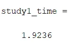
study1_time = toc

figure(1);
subplot(2,1,1);
hold on
surfc(x, y, g);
shading interp;
plot3(xopt, yopt, fopt, 'marker', 'o', 'markersize', 5, 'markerfacecolor', 'r');
title('unbounded inputs');
subplot(2,1,2);
plot(fopt);
xlabel('Iterations');
ylabel('Function minimum');

%Study 2- with upper and lower bounds
tic
for i = 1:num_cases
    [inputs, fopt(i)] = ga(@stalagmite,2,[],[],[],[],[0;0],[1;1]); %0<=x,y<=1 [0;0] is lb
    xopt(i) = inputs(1);
    yopt(i) = inputs(2);
end

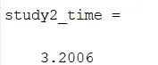
study2_time = toc

figure(2);
subplot(2,1,1);
hold on
surfc(x, y, g);
shading interp;
plot3(xopt, yopt, fopt, 'marker', 'o', 'markersize', 5, 'markerfacecolor', 'r');
title('bounded inputs');
subplot(2,1,2);
plot(fopt);
xlabel('Iterations');
ylabel('Function minimum');

%Study 3- with increased iterations
options = optimoptions('ga');
options = optimoptions(options, 'PopulationSize', 300);

tic
for i = 1:num_cases
    [inputs, fopt(i)] = ga(@stalagmite,2,[],[],[],[],[0;0],[1;1],[],[],options);
    xopt(i) = inputs(1);
    yopt(i) = inputs(2);
end

study3_time = toc

figure(3);
subplot(2,1,1);
hold on
surfc(x, y, g);
shading interp;
plot3(xopt, yopt, fopt, 'marker', 'o', 'markersize', 5, 'markerfacecolor', 'r');
title('bounded inputs with increased Population size');
subplot(2,1,2);
plot(fopt);
xlabel('Iterations');
ylabel('Function minimum');

fprintf('the maximum value of the f function is %d\n',-fopt(1));

% f = -g;
% surf(xx,yy,f);
% xlabel('x value');
% ylabel('y value');
% shading interp
% 
% [inputs, fval] = ga(@stalagmite,2);
% fval = -fval;
% fprintf('The x,y,z cordinates of the maxima of f are\n x = %d\n y = %d\n z = %d\n',inputs(1),inputs(2),fval);

% stalagamite function
function [f] = stalagmite(inp)

x = inp(1);
y = inp(2);

f1x = (sin(5.1*pi*x + 0.5))^6;
f1y = (sin(5.1*pi*y + 0.5))^6;
f2x = exp( -4*log(2)*((x-0.0677)^2)/0.64);
f2y = exp( -4*log(2)*((y-0.0677)^2)/0.64);
f = -f1x*f2x*f1y*f2y; % inverting the function
end

Output:-

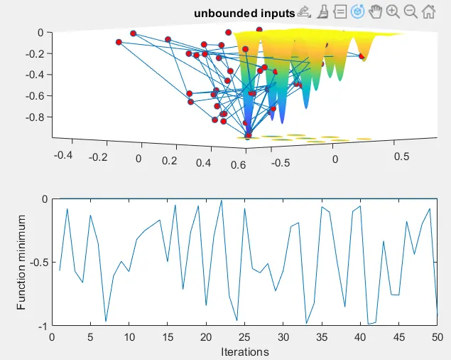
Study-1:

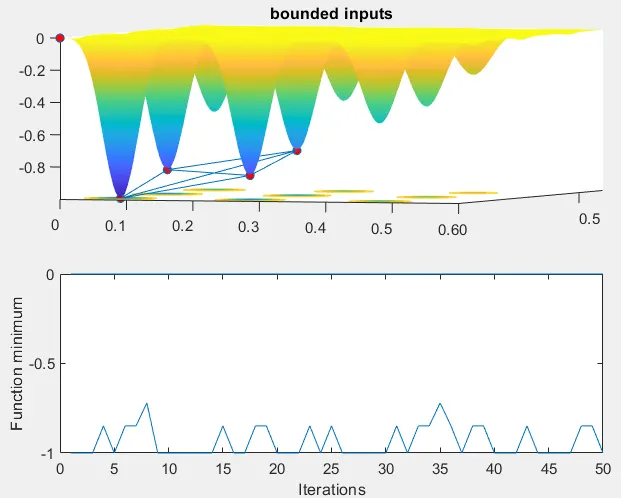
Study 2:

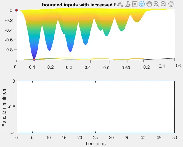
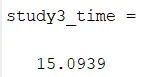
Study 3:

here the population size was increased to 300

Explanation:

 

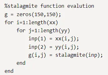
inp is an array that stores one value each of xx and yy. g is calculated for every point on the formed meshgrid.

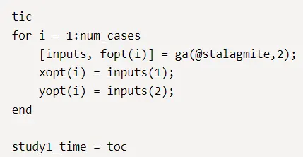
genetic algorithm is iterated for 50 times and the x,y coordinates are stored in xopt, yopt respectively.

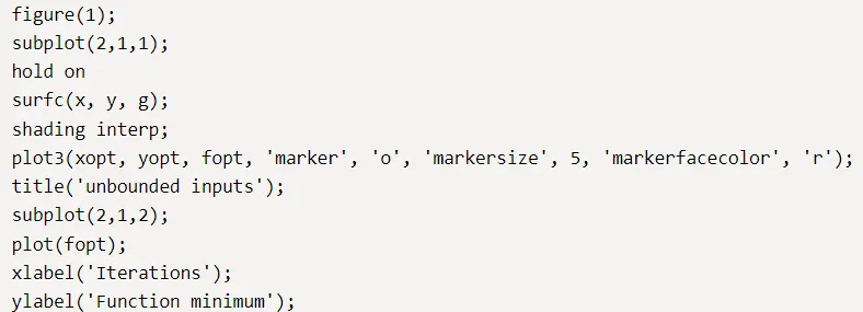
in the figure 1, the plot is divided into 2 subplots. One subplot will be marking the location of minimas in the 3D plot and the other plot will show just the value of the minimas in a 2D plot. surfc Combination surf/contour plot.

to hide the mesh over the surface, shading interp is used.

x = ga(fun,nvars,A,b,Aeq,beq,lb,ub) finds a local minimum of x function, subject to the linear equalities Aeq*x = beq and inequality A*x ≤ b so that a solution is found in the range lb ≤ x ≤ ub. All the parameters which are not defined are replaced by []

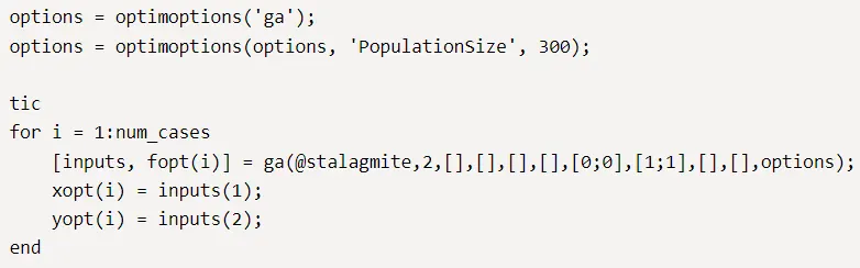
optimoptions- Create/modify optimization options. first options was created for 'ga' and then it was edited by increasing the polulation size to 300.

x = ga(fun,nvars,A,b,[],[],lb,ub,nonlcon,IntCon,options) in addition to the previous defination subjects the minimization to the constraints defined in nonlcon, minimizes with the default optimization parameters replaced by values in options. All the parameters which are not defined are replaced by []

here the f function is inverved because ga can only find minima for a function so to find the maxima for the function -f. The maxima of the function f has the same value as the minima of the function -f.

brief theory behind genetic algorithm:

Genetic algorithms are based on the ideas of natural selection and genetics. Three kinds of operations happen in genetic algorithm namely selection operation, crossover operation and mutation. Here the crossover operation is a random process therefore genetic algorithm generates random results on small iterations. 

Once the fitness scores produced having no significant difference from previous fitness scores produced by previous populations, the population is converged. The algorithm is said to be converged to a set of solutions for the problem.

By doing multiple iterations, the solutions of the genetic algorithm become better untill convergence.

The case 1 shows how chaotic it can be when the inputs are not bound by limits. The case 2 gives much better results just by defining bounds for inputs. The case 3 increases the size of the population because in lesser population just the local minimas. To get the global minima, the population is increased.