Week 3 - Taylor table method and Matlab code

for CDS

∂^2f(x)/∂x^2=af(i)+bf(i-1)+cf(i-2)+df(i+1)+ef(i+2)

for Skewed right side

∂^2f(x)/∂x^2=af(i)+bf(i+1)cf(i+2)+df(i+3)+e(i+4)

for Skewed left side

∂^2f(x)/∂x^2=af(i)+bf(i-1)cf(i-2)+df(i-3)+e(i-4)

equations formed from cds

a+b+c+d+e=0 (coefficient of f(x))

-b-2c+d+2e=0(coefficient of f'(x))

.5b+2c+.5d+2e=1(coefficient of f''(x))

-b-8c+d+8e=0(coefficient of f'''(x))

b+16c+d+16e=0(coefficient of f''''(x))

this was solved in the following code to get values for a,b,c,d,e by usingC=inv(A)*(B)

equations formed from skewed (right and left)

NOTE:THE Equations for both left and right will be the same and the coefficients also.

a+b+c+d+e=0 (coefficient of f(x))

b+2c+3d+4e=0(coefficient of f'(x))

b+2c+4.5d+8e=1(coefficient of f''(x))

b+8c+27d+64e=0(coefficient of f'''(x))

b+16c+81d+256e=0(coefficient of f''''(x))

this was solved in the following code to get values for a,b,c,d,e by usingF=inv(D)*E

these equations were derived by using taylor series expansion for each term.

CODE:

A=[1 1 1 1 1;0 -1 -2 1 2;0 0.5 2 0.5 2;0 -1 -8 1 8;0 1 16 1 16]
B=[0; 0 ;1; 0; 0]
C=inv(A)*B
D=[1 1 1 1 1; 0 1 2 3 4;0 0.5 2 4.5 8;0 1 8 27 64;0 1 16 81 256]
E=[0; 0; 1 ;0; 0]
F=inv(D)*E
syms x
f(x)=exp(x)*cos(x)
g(x)=(diff(diff(f(x),x),x))
actual=vpa(g(pi/3))
dx=vpa(linspace(pi/4,pi/4000,80))
centralordr=zeros(1,80)
skewedright=zeros(1,80)
skewedleft=zeros(1,80)
central_order_error=zeros(1,80)
skewedright_order_error=zeros(1,80)
skewedleft_order_error=zeros(1,80)
for i=1:length(dx)
    
centralordr(i)=vpa(-2.5*f(pi/3)+1.33*f(pi/3-dx(i))-0.0833*f((pi/3)-(2*dx(i)))+1.333*f(pi/3+dx(i))-0.0833*f(pi/3+(2*dx(i))))
skewedright(i)=vpa(2.9167*f(pi/3)-8.667*f(pi/3+dx(i))+9.500*f(pi/3+(2*dx(i)))-4.667*f(pi/3+(3*dx(i)))+0.9167*f(pi/3+(4*dx(i))))
skewedleft(i)=vpa(2.9167*f(pi/3)-8.667*f(pi/3-dx(i))+9.500*f(pi/3-(2*dx(i)))-4.667*f(pi/3-(3*dx(i)))+0.9167*f(pi/3-(4*dx(i))))   
central_order_error(i)=vpa(abs(actual-centralordr(i)))
skewedright_order_error(i)=vpa(abs(actual-skewedright(i)))
skewedleft_order_error(i)=vpa(abs(actual-skewedleft(i)))
end
loglog(dx,central_order_error)
hold on
loglog(dx,skewedright_order_error)
hold on
loglog(dx,skewedleft_order_error)
hold off
legend("central_order_error","skewedright_order_error","skewedleft_order_error")
xlabel("dx")
ylabel("absolute error")

OUTPUT:

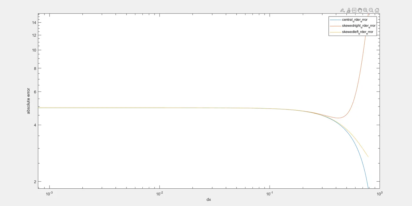
Explanation of graph:

The graph shows that the error is maximum in skewed right and minmum in CDS but somewhere in between in skewed left scheme.

If we find the value of a property or scalar field at boundary we cannot use CDS because we need to know the value at left and right of boundary so for that we use skewed schemes.We can use forward difference or backward difference scheme for boundary value problem but they would not be as accurate as skewed scheme as it is of order 4 approx.

Proof of fourth order approximation:

∂^2f(x)/∂x^2=af(i)+bf(i+1)cf(i+2)+df(i+3)+e(i+4)

now

∂^2f(x)/∂x^2=(b+2c+4.5d+8e)f"(x)(dx)^2+(dx)^6f"""(x)

now

f"""(x)(dx)^6

a 0

b 1/720

c 64/720

d 243/720

e 1024/720

so considering some finite value of

the coefficients

∂^2f(x)/∂x^2=(af(i)+bf(i+1)cf(i+2)+df(i+3)+e(i+4))/(dx)^2=kf"(x)+O(dx)^4

here k=b+2c+4.5d+8e)

so the skewed schemes are of order 4.