Week 3 - Taylor table method and Matlab code

Aim : Taylor table method and Matlab code

Objective :

1. Deriving the following 4th order approximations of the second-order derivative for central difference, skewed right-sided difference and skewed left-sided difference.

2. Prove that skewed schemes are fourth-order accurate.

3. Write a program in Matlab to evaluate the second-order derivative of the analytical function exp(x)*cos(x)

4. Compare it with the 3 numerical approximations.

Procedure :

1)For given Analytical function f(x)= exp(x)*cos(x), Analytical derivative will be f''(x)= -(2*exp(x)*sin(x))

2) Formulation of derivative for central difference,left and right skewed errors

Matlab Code :

• Function for first order approximation

function value = skewed_RS_approximation(x,dx)

%Analytical derivative
%f(x) = exp(x)*cos(x)
%f''(x) = -(2*exp(x)*sin(x))
analytical_derivative = -(2*exp(x)*sin(x));

A = [1 1 1 1 1 1
    0 1 2 3 4 5 
    0 1/2 2 9/2 8 25/2
    0 1/6 4/3 9/2 32/3 125/6
    0 1/24 2/3 27/8 32/3 625/24
    0 1/120 4/15 81/40 128/15 625/24]

B = [0
     0
     1
     0
     0
     0]
 
X = inv(A)*B
 %Using central difference of first order derivative
 skewed_RS_difference = (X(1)*(exp(x)*cos(x))+X(2)*(exp(x+dx)*cos(x+dx))+X(3)*(exp(x+2*dx)*cos(x+2*dx))+X(4)*(exp(x+3*dx)*cos(x+3*dx))+X(5)*(exp(x+4*dx)*cos(x+4*dx))+X(6)*(exp(x+5*dx)*cos(x+5*dx)))/(dx)^2;
 
 value = abs(skewed_RS_difference - analytical_derivative);
end

• Function for second order approximation

function value = skewed_LS_approximation(x,dx)

%Analytical derivative
%f(x) = exp(x)*cos(x)
%f''(x) = -(2*exp(x)*sin(x))
analytical_derivative = -(2*exp(x)*sin(x));

A = [ 1 1 1 1 1 1
      -5 -4 -3 -2 -1 0
      25/2 8 9/2 2 1/2 0
      -125/6 -32/3 -9/2 -4/3 -1/6 0
      625/24 32/3 27/8 2/3 1/24 0
      -625/24 -128/15 -81/40 -4/15 -1/120 0]

B = [0
     0
     1
     0
     0
     0]
 
X = inv(A)*B
%Using central difference of second order derivative
skewed_LS_difference =(X(1)*(exp(x-5*dx)*cos(x-5*dx))+X(2)*(exp(x-4*dx)*cos(x-4*dx))+X(3)*(exp(x-3*dx)*cos(x-3*dx))+X(4)*(exp(x-2*dx)*cos(x-2*dx))+X(5)*(exp(x-dx)*cos(x-dx))+X(6)*(exp(x)*cos(x)))/(dx)^2;

value = abs(skewed_LS_difference - analytical_derivative );
end

• Function for fourth order approximation

function value = central_approximation(x,dx)

%Analytical derivative
%f(x) = exp(x)*cos(x)
%f''(x) = -(2*exp(x)*sin(x))
analytical_derivative = -(2*exp(x)*sin(x));
A = [1 1 1 1 1
    -2 -1 0 1 2
    2 1/2 0 1/2 2
    -4/3 -1/6 0 1/6 4/3
    2/3 1/24 0 1/24 2/3]

B = [0
     0
     1
     0
     0]

X = inv(A)*B


%Using central difference of fourth order derivative
central_difference= (X(1)*(exp(x-2*dx)*cos(x-2*dx))+X(2)*(exp(x-dx)*cos(x-dx))+X(3)*(exp(x)*cos(x))+X(4)*(exp(x+dx)*cos(x+dx))+X(5)*(exp(x+2*dx)*cos(x+2*dx)))/(dx)^2;

value = abs(central_difference - analytical_derivative );
end

Main code :

The above three functions are formulated as approximation errors, these three are called in the main code to calculate the error over a given range of dx

clear all 
close all 
clc

%Inputs
x = pi/4;
dx = linspace(pi/4,pi/40000,100);
%Analytical_derivative
%f(x)= exp(x)*cos(x)
%f''(x)= -(2*exp(x)*sin(x))
%Calculation of 4th order approxmation of the second order
%derivative for central difference,left and right skewed errors
for i = 1:length(dx)
    analytical_derivative = -(2*exp(x)*sin(x));
    central_difference_error(i) = central_approximation(x,dx(i));
    skewed_LS_difference_error(i) = skewed_LS_approximation(x,dx(i));
    skewed_RS_difference_error(i) = skewed_RS_approximation(x,dx(i));
end



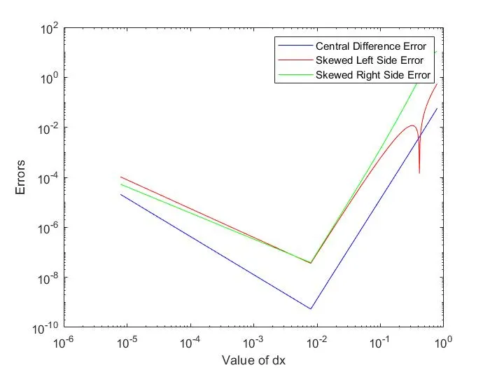
%Comparing errors using Graph
figure(1)
loglog(dx,central_difference_error,'color','b')
hold on
loglog(dx,skewed_LS_difference_error,'color','r')
hold on
loglog(dx,skewed_RS_difference_error,'color','g')

legend('Central Difference Error','Skewed Left Side Error','Skewed Right Side Error')
xlabel ('Value of dx')
ylabel ('Errors')

Outputs :

Output of central difference of fourth order derivative

A =

    1.0000    1.0000    1.0000    1.0000    1.0000
   -2.0000   -1.0000         0    1.0000    2.0000
    2.0000    0.5000         0    0.5000    2.0000
   -1.3333   -0.1667         0    0.1667    1.3333
    0.6667    0.0417         0    0.0417    0.6667


B =

     0
     0
     1
     0
     0


X =

   -0.0833
    1.3333
   -2.5000
    1.3333
   -0.0833

Output of skewed LS difference of second order derivative
A =

    1.0000    1.0000    1.0000    1.0000    1.0000    1.0000
   -5.0000   -4.0000   -3.0000   -2.0000   -1.0000         0
   12.5000    8.0000    4.5000    2.0000    0.5000         0
  -20.8333  -10.6667   -4.5000   -1.3333   -0.1667         0
   26.0417   10.6667    3.3750    0.6667    0.0417         0
  -26.0417   -8.5333   -2.0250   -0.2667   -0.0083         0


B =

     0
     0
     1
     0
     0
     0


X =

   -0.8333
    5.0833
  -13.0000
   17.8333
  -12.8333
    3.7500

Output of skewed LS difference of second order derivative
A =

    1.0000    1.0000    1.0000    1.0000    1.0000    1.0000
         0    1.0000    2.0000    3.0000    4.0000    5.0000
         0    0.5000    2.0000    4.5000    8.0000   12.5000
         0    0.1667    1.3333    4.5000   10.6667   20.8333
         0    0.0417    0.6667    3.3750   10.6667   26.0417
         0    0.0083    0.2667    2.0250    8.5333   26.0417


B =

     0
     0
     1
     0
     0
     0


X =

    3.7500
  -12.8333
   17.8333
  -13.0000
    5.0833
   -0.8333

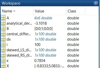
Workspace :

Graph :

Conclusion :

1) From the above graph it can be said that error increases by increasing the Value of dx

2) At some point of time we can see that the errors increases exponentially.

3) For 1st and 2nd order errors it is observed that both are in same line and at certain point their error is variable.

4) Accuracy is observed in the fourth order approximation which is caused due to the lesser value of error with respect to the value of dx.