Week 3 - Taylor table method and Matlab code

Abstract: To derive the fourth-order of the second derivative with the central, skewed right, and skewed left differencing for the function f(x)=exp(x)*cos(x).

Central differencing with fourth-order approximation:

`(del^2f)/(delx^2) approx(f''(x)+Deltax^4f^6)/(Deltax^2)=(af(i)+bf(i+1)+c(i+2)+d(i-1)+e(i-2))/(Deltax^2)`

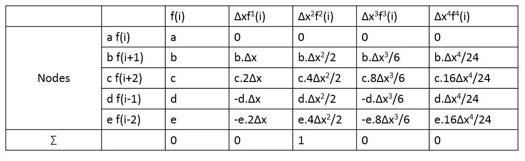
By solving the above equations using octave the coefficients found is below:

a=-2.5, b=1.3333, c=-0.0833, d=1.3333 & e=-0.0833

Octave function coded using the above coefficients to calculate error by comparing analytical vs central differencing:

function error = Fourth_Order_Central_Approximation(x,dx)
% analytical function is f(x)=exp(x)*cos(x)
% analytical derivative 
% f''(x) = -2*exp(x)*sin(x);
analytical_derivative= -2*exp(x)*sin(x);
central_differencing=((-0.0833*cos(x-2*dx)*exp(x-2*dx))+(1.3333*cos(x-dx)*exp(x-dx))+(-2.5*cos(x)*exp(x))+(1.3333*cos(x+dx)*exp(x+dx))+(-0.0833*cos(x+2*dx)*exp(x+2*dx)))/dx^2;
error = abs(central_differencing-analytical_derivative);
end

Skewed Right differencing with fourth order approximation:

`(del^2f)/(delx^2) approx(f''(x)+Deltax^4f^6)/(Deltax^2)=(af(i)+bf(i+1)+c(i+2)+d(i+3)+e(i+4)+g(i+5))/(Deltax^2)`

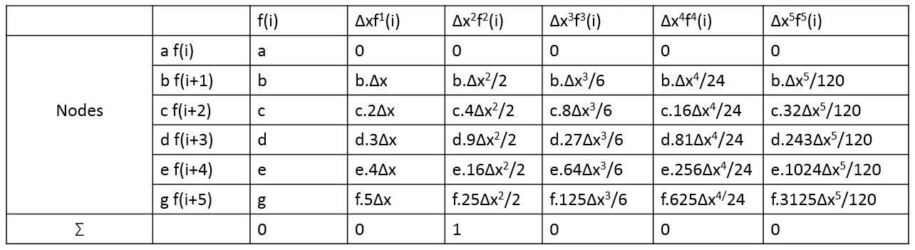
By solving the above equations using octave the coefficients found is below:

a=3.75, b=-12.8333, c=17.8333, d=13, e=5.0833 & g=-0.8333

Octave function coded using the above coefficients to calculate error by comparing analytical vs skewed right differencing:

function error = Fourth_Order_Skewed_Right_Approximation(x,dx)
% analytical function is f(x)=exp(x)*cos(x)
% analytical derivative 
% f''(x) = -2*exp(x)*sin(x);
analytical_derivative= -2*exp(x)*sin(x);
skewed_right_differencing=((3.75*cos(x)*exp(x))+(-12.8333*cos(x+dx)*exp(x+dx))+(17.8333*cos(x+2*dx)*exp(x+2*dx))+(-13*cos(x+3*dx)*exp(x+3*dx))+(5.0833*cos(x+4*dx)*exp(x+4*dx))+(-0.8333*cos(x+5*dx)*exp(x+5*dx)))/dx^2;
error = abs(skewed_right_differencing-analytical_derivative);
end

Skewed Right differencing with fourth order approximation:

`(del^2f)/(delx^2) approx(f''(x)+Deltax^4f^6)/(Deltax^2)=(af(i)+bf(i-1)+c(i-2)+d(i-3)+e(i-4)+g(i-5))/(Deltax^2)`

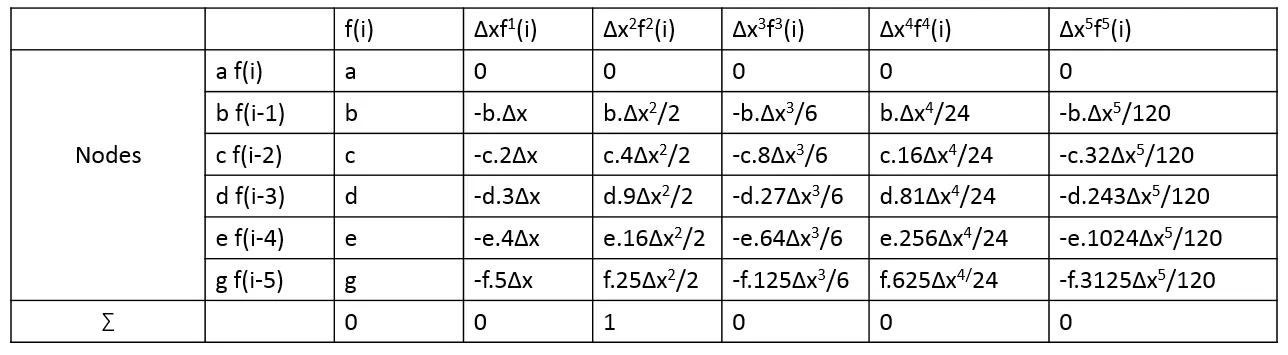
By solving the above equations using octave the coefficients found is below:

a=3.75, b=-12.8333, c=17.8333, d=13, e=5.0833 & g=-0.8333

Octave function coded using the above coefficients to calculate error by comparing analytical vs skewed left differencing:

function error = Fourth_Order_Skewed_Left_Approximation(x,dx)
% analytical function is f(x)=exp(x)*cos(x)
% analytical derivative 
% f''(x) = -2*exp(x)*sin(x);
analytical_derivative= -2*exp(x)*sin(x);
skewed_left_differencing=(3.75*cos_x(x)-12.833*cos_x(x-dx)+17.8333*cos_x(x-2*dx)-13*cos_x(x-3*dx)+5.0833*cos_x(x-4*dx)-0.833*cos_x(x-5*dx))/dx;
error = abs(skewed_left_differencing-analytical_derivative);
end

Octave function to calculate the accuracy of the skewed fourth order approximation:

clear all
close all
clc
x=pi/3
dx=linspace(pi/20,pi/1000,20)
for i=1:length(dx)
  second_central_order_error(i)=Fourth_Order_Central_Approximation(x,dx(i));
  second_skewed_right_order_error(i)=Fourth_Order_Skewed_Right_Approximation(x,dx(i));
  second_skewed_left_order_error(i)=Fourth_Order_Skewed_Left_Approximation(x,dx(i));
end
figure(1)
%plot(dx,second_central_order_error)
loglog(dx,second_central_order_error)
hold on
loglog(dx,second_skewed_right_order_error)
hold on
loglog(dx,second_skewed_left_order_error)
xlabel('dx')
ylabel('error')
legend('Central Error', 'Right Error', 'Left Error')
title('Comparison of error for central, skewed right and skewed left approximation')

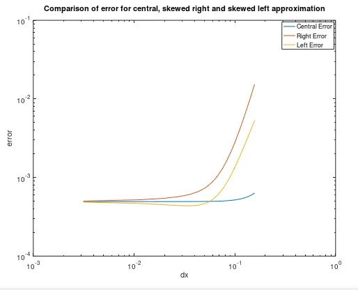
The plot shows the absolute error with respect to analytical derivative.

Conclusion:

The above plot clearly central differencing shows a minimal percentage of error and consistent compared to the other differencing.

But skewed matrix is needed wherever central differencing is not possible usually at the boundaries.