Taylor table method and Matlab code

Introduction:

The numerical solutions can only give answers at discrete points in the domain which are called as grid points. The finite difference method is for replacing the partial derivates appearing in the governing equation of fluid dynamics, with algebraic difference quotients yeilding a system of governing equations that can be solved for the flow field variables at the specific discrete grid points in the flow.

Schemes for fourth-order approximations for second-order derivatives:

We have a set of grid points in our numerical stencil along the x-plane. Each grid point has its own Taylor series functions. We first create a Taylor table from this set of grid points as shown below.

Central difference scheme:

central differencing with fourth order approximation:

af(i−2)+bf(i−1)+c

	f(i)	f'(i)*ΔΔ(x)	f''(i)*ΔΔ(x)^2	f'''(i)*ΔΔ(x)^3	f''''(i)*ΔΔ(x)^4
f(i-2)	a	-2a	4a/2	-8a/6	16a/24
f(i-1)	b	-b	b/2	-b/6	b/24
f(i)	c	0	0	0	0
f(i+1)	d	d	d/2	d/6	d/24
f(i+2)	e	2e	4e/2	8e/6	16e/24
	0	0	1	0	0

Matlab code
E=[1 1 1 1 1;
    -2 -1 0 1 2;
    4/2 1/2 0 1/2 4/2;
    -8/6 -1/6 0 1/6 8/6;
    16/24 1/24 0 1/24 16/24];

F=[0;0;1;0;0];

Z=rats(linsolve(E,F))

Outputs:

Skewed right-sided difference scheme:

skewed right sided with fourth order approximation:

af(i)+bf(i+1)+cf(i+2)+d

	f(i)	f'(i)*ΔΔ(x)	f''(i)*ΔΔ(x)^2	f'''(i)*ΔΔ(x)^3	f''''(i)*ΔΔ(x)^4	f'''''(i)*ΔΔ(x)^5
f(i)	a	0	0	0	0	0
f(i+1)	b	b	b/2	b/6	b/24	b/120
f(i+2)	c	2c	4c/2	8c/6	16c/24	32c/120
f(i+3)	d	3d	9d/2	27d/6	81d/24	243d/120
f(i+4)	e	4e	16e/2	64e/6	256e/24	1024e/120
f(i+5)	g	5g	25g/2	125g/6	625g/24	3125g/120
	0	0	1	0	0	0

Matlab code

E=[1 1 1 1 1 1;
    0 1 2 3 4 5 ;
    0 1/2 4/2 9/2 16/2 25/2;
    0 1/6 8/6 27/6 64/6 125/6;
    0 1/24 16/24 81/24 256/24 625/24;
    0 1/120 32/120 243/120 1024/120 3125/120];

F=[0;0;1;0;0;0];
Z=rats(linsolve(E,F))

Outputs:

3.Skewed left-sided difference scheme:

	f(i)	f'(i)*ΔΔ(x)	f''(i)*ΔΔ(x)^2	f'''(i)*ΔΔ(x)^3	f''''(i)*ΔΔ(x)^4	f'''''(i)*ΔΔ(x)^5
f(i)	a	0	0	-0	0	-0
f(i-1)	b	-b	b/2	-b/6	b/24	-b/120
f(i-2)	c	-2c	4c/2	-8c/6	16c/24	-32c/120
f(i-3)	d	-3d	9d/2	-27d/6	81d/24	-243d/120
f(i-4)	e	-4e	16e/2	-64e/6	256e/24	-1024e/120
f(i-5)	g	-5g	25g/2	-125g/6	625g/24	-3125g/120
	0	0	1	0	0	0

Matlab code

E=[1 1 1 1 1 1;
    0 -1 -2 -3 -4 -5 ;
    0 1/2 4/2 9/2 16/2 25/2;
    0 -1/6 -8/6 -27/6 -64/6 -125/6;
    0 1/24 16/24 81/24 256/24 625/24;
    0 -1/120 -32/120 -243/120 -1024/120 -3125/120];

F=[0;0;1;0;0;0];
Z=rats(linsolve(E,F))

Outputs:

Derivates:

Analytical_derivative =exp(x)*((cos(x)-sin(x))-(cos(x)+(sin(x))));

Forward_differencing =((15/4*cos_x(x))-(77/6*cos_x(x+1*dx))+(107/6*cos_x(x+2*dx))-(13*cos_x(x+3*dx))+(61/12*cos_x(x+4*dx))-(5/6*cos_x(x+5*dx)))/dx^2;

Backward_differencing =((15/4*cos_x(x))-(77/6*cos_x(x-1*dx))+(107/6*cos_x(x-2*dx))-(13*cos_x(x-3*dx))+(61/12*cos_x(x-4*dx))-(5/6*cos_x(x-5*dx)))/dx^2;

Central_differencing =((-1/12*cos_x(x-2*dx))+(4/3*cos_x(x-1*dx))-(5/2*cos_x(x))+(4/3*cos_x(x+1*dx))-(1/12*cos_x(x+2*dx)))/dx^2;

Creating functions for cos_x

function [xdot]= cos_x(x)

xdot=(exp(x)*cos(x));

end

Skewed right-sided approximation function:

function out=rightskew_approximation(x,dx)

%analytical derivation
%f'(x)=exp(x)*((cos(x)-sin(x))-(cos(x)+(sin(x))));
analytical_derivative =exp(x)*((cos(x)-sin(x))-(cos(x)+(sin(x))));

%numerical derivative
forward_differencing =((15/4*cos_x(x))-(77/6*cos_x(x+1*dx))+(107/6*cos_x(x+2*dx))-(13*cos_x(x+3*dx))+(61/12*cos_x(x+4*dx))-(5/6*cos_x(x+5*dx)))/dx^2;

out=abs(forward_differencing - analytical_derivative);

end

Skewed left-sided approximation function:

function out=leftskew_approximation(x,dx)

%analytical derivation
%f'(x)=exp(x)*((cos(x)-sin(x))-(cos(x)+(sin(x))));
analytical_derivative =exp(x)*((cos(x)-sin(x))-(cos(x)+(sin(x))));

%numerical derivative
backward_differencing =((15/4*cos_x(x))-(77/6*cos_x(x-1*dx))+(107/6*cos_x(x-2*dx))-(13*cos_x(x-3*dx))+(61/12*cos_x(x-4*dx))-(5/6*cos_x(x-5*dx)))/dx^2;

out=abs(backward_differencing - analytical_derivative);

end

Central difference approximation function:

function out=centraldiff_approximation(x,dx)

%analytical derivation
%f'(x)=exp(x)*((cos(x)-sin(x))-(cos(x)+(sin(x))));
analytical_derivative =exp(x)*((cos(x)-sin(x))-(cos(x)+(sin(x))));

%numerical derivative
central_differencing =((-1/12*cos_x(x-2*dx))+(4/3*cos_x(x-1*dx))-(5/2*cos_x(x))+(4/3*cos_x(x+1*dx))-(1/12*cos_x(x+2*dx)))/dx^2;

out=abs(central_differencing - analytical_derivative);

end

MATLAB coding

%Taylor table
clear all 
close all
clc
 
x = pi/3;

dx = linspace(pi/4,pi/400,20);

for i = 1:length(dx)
    
    rightskew_error(i)=rightskew_approximation(x,dx(i));
    
    leftskew_error(i)=leftskew_approximation(x,dx(i));
    
    centraldiff_error(i)=centraldiff_approximation(x,dx(i));
    
end

%Plotting
loglog(dx,rightskew_error,'g')
hold on
loglog(dx,leftskew_error,'b')
loglog(dx,centraldiff_error,'r')
hold off
xlabel('values of dx')
ylabel('errors')
legend('rightskew','leftskew','centraldiff')

Result:

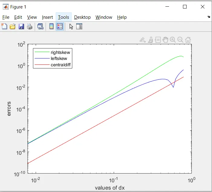
As we can see from the above figure the error for the central difference method is very less compared to the skewed methods.

Skewed right and left difference methods almost gives the same results in terms of error for a small value of time step.

Describe why a skewed scheme is useful? What can a skewed scheme do that a CD scheme cannot?

Because in some complex system the numerical stencil wont be symmetric points is available and at this point only skewed scheme can help. And the advantage of using skewed system is seen near the boundaries where there is no access to further points over the boundary i,e Asymmetric.

Skewed schemes utilize data from either left or right data points from the point of consideration,whereas central difference scheme us data from both left and right from the point of consideration.