Week 3 - Solving second order ODEs

Solving second order ODEs

Aim:

• To write a program to solve the ODE that simulates a pendulum.

Project Objectives:

• To solve ODE of pendulum using ‘ode45’ function.
• To represent the equation of motion of a simple pendulum with damping.
• To plot graph showing angular displacement and velocity for specific time-span.
• To animate the motion of pendulum.’

Background:

In Engineering, ODE is used to describe the transient behaviour of a system. A simple example is a pendulum. The way the pendulum moves depends on the Newtons second law. When this law is written down, we get a second order Ordinary Differential Equation that describes the position of the "ball" w.r.t time. Similarly, there are hundreds of ODEs that describe key phenomena. If we have the ability to solve these equations, we will also be able to simulate the respective phenomena.

Governing equations:

The equation of motion of a simple pendulum with damping is as follows:

In the above equation,

Θ = angular displacement in rad

t = time in sec

g = gravity in m/sec^2

L = length of the pendulum in m,

m = mass of the ball in kg,

b = damping coefficient.

We get the position and velocity of pendulum as a function of time.

Code:

1) Main code:

clc
clear all
close all

%inputs
l = 1;     %length_of_pendulam (m)
m = 1;     %mass_ of_ball (kg)
b = 0.05;  %damping_coefficient 
g = 9.81;  %gravity (m/sec^2)

%initial conditions of pendulam
theta_0 = [0; 3];   %displacement = 0 rad, velocity = 3 rad/sec

%timespan
t_span = [0:0.1:20]; %from 0-20 seconds

%solving ODE
[t, results] = ode45(@(t, theta) ode_func1(t, theta, b, g, l, m), t_span, theta_0)
  
figure(1)
%plotting graph
plot(t, results(:, 1)); %plots_values_of_1st_column_of_results_ie_angular_displacement
hold on;
plot(t, results(:, 2)); %plots_values_of_2nd_column_of_results_ie_angular_velocity
xlabel('Time');
ylabel('Displacement/Velocity');
grid on;

%creating animation
ct = 1;
angu_disp = results(:, 1);   %storing_values_of_angular_displacement
for i = [1:length(angu_disp)]; 
    THETA = angu_disp(i);
    
    %setting coordnate values of pendulam string
    
    x0 = 0;
    y0 = 0;
    
    x1 = l*sin(THETA);
    y1 = -l*cos(THETA);
    
    figure(2)
   
    plot([-1 1], [0 0],[x0 x1],[y0 y1], 'linewidth', 3); %plotting horizontal line and pendulam string
    hold on;
    %attaching pendulam sphere to string
    plot(x1, y1, 'Marker', 'O', 'MarkerSize', 30, 'MarkerEdgeColor', 'red', 'MarkerFaceColor', [1 0 0]);
    hold off;
    axis([-1.5 1.5 -1.5 1.5]);
    pause(0.08);
    
     %saving_individual_frame
        M(ct) = getframe(gcf);      %save_each_figure_of_graph_as_a_frame
        ct = ct + 1;
    

end

%creating_and_saving_movie_file
movie(M);                           %generate_movie_of_all_frames_stored_in_M
video_file = VideoWriter('solving_ODE_1.avi', 'uncompressed AVI'); %creates_video_file
open(video_file);
writeVideo(video_file, M);
close(video_file);

2) Function code:

function [dtheta_dt] = ode_func1(t, theta, b, g, l, m)
theta1 = theta(1);
theta2 = theta(2);
dtheta1_dt = theta2;
dtheta2_dt = -[b/m]*theta2 - [g/l]*sin(theta1);
dtheta_dt = [dtheta1_dt; dtheta2_dt];   

end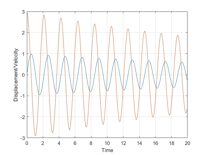

Angular displacement and velocity plot against time.

First, we give input values of pendulum equations. Then we specify the initial conditions and time span. The pendulum equation is solved by using ‘ode45@’ solver which is based on Runge-Kutta method. To solve this Second order equation, we first transform it into first order function which gives us 2 variables of 1^st order. This is done in a separate function code and this function is called in the main code. When this equation is solved, we get the results in 2 columns; first one gives angular displacement and second gives angular velocity at respective time intervals mentioned in time span.

The values of displacement and velocity of pendulum are plotted against time. We get an alternating sinusoidal plot. This plot drastically changes its shape if damping coefficient is varied.

Then, for creating animation of pendulum, we make use of ‘for loop’, where we get figures of each position of pendulum. These figures are stored in variable ‘M’ in form of frames. Then using these frames, a video clip is made and saved in the folder.

Animation link:

https://youtu.be/iD3rFkpq5iM

Conclusion:

• Ode45 solver can be used to perform simulation by showing the solution as it changes in time.
• From angular displacement and velocity plot, it can be seen that the displacement-velocity fluctuations or vibrations are damped quickly by increase in damping coefficient value.
• Results from solving ODEs can be used for plotting and simulating a phenomenon.