Week 3 - Solving second order ODEs

AIM: Write a program to simulate the behavior of a simple pendulum and to create an animation of its motion.

INTRODUCTION:

A simple pendulum is defined to have a small mass, also known as the pendulum bob, which is suspended from a light wire or string.

In Engineering ODE is used to describe the transient behaviour of a system. A simple example is a pendulum. The way the pendulum moves depends on Newton's second law. When this law is written down, we get a second-order Ordinary Differential Equation that describes the position of the "ball".

ODE represents the equation of motion of a simple pendulum with damping

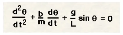
In the above equation,

g = gravity in m/s2,

L = length of the pendulum in m,

m = mass of the ball in kg,

b=damping coefficient.

Write a program in Python that will simulate the pendulum motion, just like the one shown in the start of this challenge.

use,

L=1 metre,

m=1 kg,

b=0.05.

g=9.81 m/s2.

Simulate the motion between 0-20 sec, for angular displacement=0,angular velocity=3 rad/sec at time t=0.

EXPLANATION OF CODE:

1. To solve ODE, import odeint module from scipy module.
2. Break down the second-order ODE into two first-order ODE, the first ODE will give the value of displacement and the second ODE will give the value of velocity.
3. Define the initial condition to solve ODE as ' theta_0 = [0,3].
4. To obtain smooth motion, drive time point between 0 to 20 sec using linspace command.
5. To solve ODE use 'ODEINT' and save values in variable 'theta'
6. theta = odeint(model,theta_0,t,args =(b,g,l,m))
7. First column of the matrix represents the values of displacement hence extract values of displacement and add it in null matrix THETA3 using append command.
8. To show the motion pf pendulum for every value of THETA3 extract values of THETA4 using loop.

CODE FOR SOLVING SECOND ORDER ODEs:

import numpy as np
from scipy.integrate import odeint
import matplotlib.pyplot as plt
import math
# function that returns dz/dt
def model (theta,t,b,g,l,m):
theta1 = theta [0]
theta2 = theta [1]
dtheta1_dt = theta2
dtheta2_dt = -(b/m)*theta2 - (g/l)*math.sin(theta1)
dtheta_dt = [dtheta1_dt,dtheta2_dt]
return dtheta_dt
#input
#damping co-efficient
b = 0.05
# gravity n m/s2
g = 9.81
# length of the pendulum in m
l = 1
# mass of the ball in kg
m = 0.1
# intial condition
theta_0 = [0,3]
# time points
t = np.linspace(0,20,150)
# solve ODE
theta = odeint(model,theta_0,t,args =(b,g,l,m))
#plot
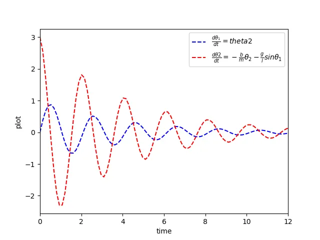
plt.plot(t,theta[:,0],'b--',label = r'$\frac{d\theta_1}{dt} = theta2 $')
plt.plot(t,theta[:,1],'r--',label = r'$\frac{d\theta2}{dt} = - \frac{b}{m}\theta_2 -\frac{g}{l}sin\theta_1 $')
plt.xlabel('time')
plt.ylabel('plot')
plt.xlim(0,12)
plt.legend(loc = 'best')
plt.show()

# animation
THETA3 = []
for theta3 in theta[:,0]:
THETA3.append(theta3)
ct = 1
for THETA4 in THETA3:
x0 = 0
y0 = 0
x1 = l*math.sin(THETA4)
y1 = -l*math.cos(THETA4)

filename = 'pendulum%05d.png'%ct
ct = ct+1
# Horizontal support or pendulum
plt.plot([-0.2,0.2],[0,0])
# string of pendulum
plt.plot([x0,x1],[y0,y1])
# Bob tied at the end
plt.plot(x1,y1,'-o')
plt.xlim([-1.5,1.5])
plt.ylim([-1.5,1])
plt.title('motion of pendulum')
plt.savefig(filename)
plt.show()

RESULT:

1. Time plot:

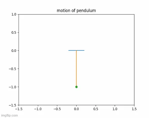
2. Animation of Motion of Pendulum:

CODE LINK:

https://drive.google.com/drive/folders/1FSDjV7SgnU-CjP79uGRmdpK7DTK4BxVJ?usp=sharing