Week 3 - Solving second order ODEs

Solving second order ODE's

Introduction :A pendulum is a body suspended from a point that is fixed so that it can swing back and forth due to gravitational forces acting on it.
They can be used in the construction odf clocks , as the time taken to complete one full oscilation(period) is a constant.This time interval has various factors affecting it,
such as :
1)Length of pendulum
2)amplitude
3)width of its swing

Aim: To solve a second order ODE depicting the motion of a pendulumand create its animation.

Objective:
To write a program to solve the following ODE.

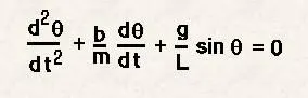
In this equation
g = gravity in m/s2
L= length of pendulum in m
m = mass of all in kg
b = damping coeffecient

Fixed Parameters:
Length(L) = 1 metre
Mass(m) = 1kg
Damping coeffecient(b) =0.05
Acceleration due to gravity (g) = 9.81m/s2
Time span = 0 - 20 seconds
Anglar displacement = 0
Angular velocity = 3rad /sec at time t = 0

Function code :

%ODE function
function dtheta_dt = ode_fun(t,theta,b,g,l,m)
theta1 = theta(1)
theta2 = theta(2)
dtheta1_dt = theta2
dtheta2_dt = -(b/m)*theta2 - (g/l)*sin(theta1)
dtheta_dt = [dtheta1_dt ; dtheta2_dt]
end

Explanation :
1) In this function , we basically convert the second order ODE to a first order ODE by introducing 2 terms theta1 and theta2
2)Then dtheta_dt gives a column matrix by differentiating theta1 and theta2

Main code:

clear all
close all
clc
%Fixed parameters
%Damping coeffecient
b = 0.05
%Acceleration due to gravity (m/s^2)
g = 9.81
%Mass in kg
m = 1
%Length in m
L= 1
%Initial condition
theta_0 = [0;3]
%Time points
tspan = linspace(0,20,100)
%Solving ODE
[t,results] = ode45(@(t,theta)functionode(t,theta,b,g,L,m),tspan,theta_0)
%Plotting
figure(1)
plot(t,results(:,1))
hold on
plot(t,results(:,2))
xlabel('time')
ylabel('theta')
legend('angular displacement','angular velocity')
hold off
%Animation
ct = 1;
for i = 1:length(results(:,1))
    x0=0
    y0=0
    x1 = L*sin(results(i,1)+pi)
    y1 =L*cos(results(i,1)+pi)
    figure(2)
    plot([x0 x1],[y0 y1],'.','color','r','MarkerSize',50)
    line([x0 x1],[y0 y1],'color','b')
    axis([-2 2  -2 2])
    hold on
    plot([-1 1],[0 0],'color','r')
    hold on
plot([-1 1] ,[0 0],'.','MarkerSize',50)

M(ct) = getframe(gcf)
hold off
ct = ct+1
end
%Creating the movie and videofile
movie(M)
videofile = VideoWriter('Pendulum.avi','uncompressed AVI')
open(videofile)
writeVideo(videofile,M)
close(videofile)

Explanation:
1) Firstly we fix the parameters such as length , mass, damping coeffecient and acceleration due to gravity
2)Then , we input time and angle
3)Now we take 200 values between 0 to 20 for tspan
4)Now ODE function is introduced
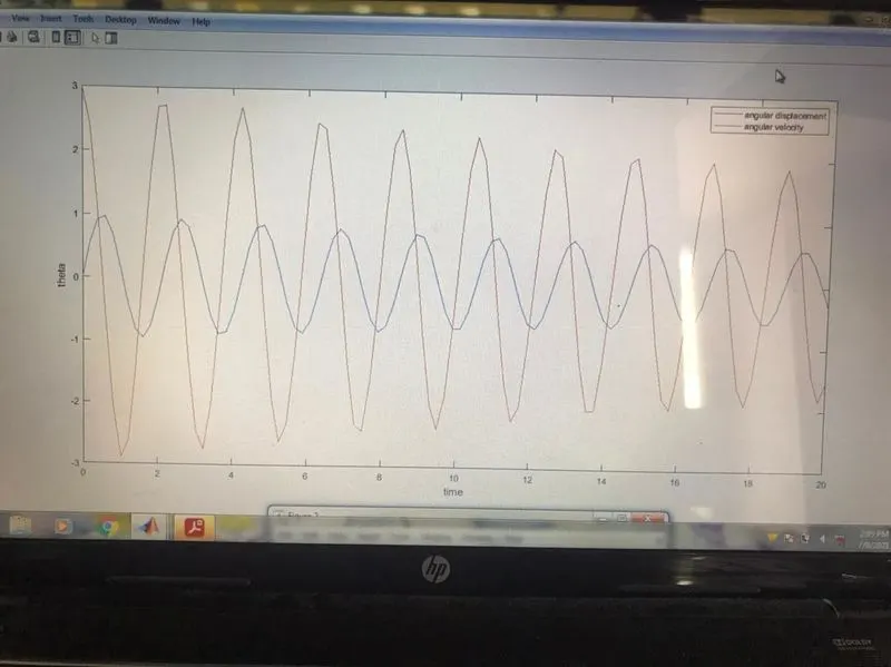
5)Using plot command ,velocity and displacement is plotted in yaxis against time in xaxis
6)Using for loop ,mass at different points t different times is plotted
7)Movie command is now used to save as an uncompressed file

Plot:

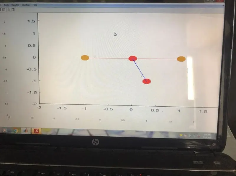
Animation (youtube link):

https://www.youtube.com/watch?v=SDREVX_2Q5s