Week 3 - Solving second order ODEs

Objective:

`(d^2theta)/dt^2 + b/m*(d theta)/dt +g/L*sin theta = 0`

g = gravity in m/s2,

L = length of the pendulum in m,

m = mass of the ball in kg,

b=damping coefficient.

A program in Python that will simulate the pendulum motion, using

L=1 metre,

m=1 kg,

b=0.05.

g=9.81 m/s2.

Simulate the motion between 0-10 sec, for angular displacement=0,angular velocity=3 rad/sec at time t=0.

"""
Second order differential equation 

by Amit Kumar
"""
import math 
from scipy.integrate import odeint
import matplotlib.pyplot as plt
import numpy as np


def second_order(theta,t,b,g,l,m):

	theta1 = theta[0]
	theta2 = theta[1]
	dtheta1_dt = theta2
	dtheta2_dt = -(b/m)*theta2 -(g/l)*(math.sin(theta1))
	dtheta_dt = [dtheta1_dt,dtheta2_dt]
	return dtheta_dt

# given data for the simple pendulum

# damping coefficien 
b = 0.02
# length of the pendulum 
l = 1
# acceleration due to gravity 
g = 9.8
# mass of the pendulum bob
m = 0.05

# initial condition
theta_0 = [0,3]

# time plot 
t = np.linspace(0,10,50)

theta = odeint(second_order,theta_0,t,args = (b,g,l,m))



plt.plot(t,theta[:,0],'b-.',label = r' Angular displacement')
plt.plot(t,theta[:,1],'r-.',label = r' Angular Velocity')
plt.xlabel('time')
plt.ylabel('plot')
plt.legend(loc ='best')
plt.title('Solve 2D order by python')
plt.show()

# Animation video of pendulum 

# initial bob position x = 0 , y = 0 
x_0 = 0
y_0 = 0 

value = []
for displ in theta[:,0]:
	value.append(displ)


ct = 1 

for i in value :
	
	x1 =  l*math.sin(i)
	y1 = - l*math.cos(i)



	filename = str(ct) +'.png'
	ct = ct + 1

	plt.figure()
	plt.plot([-1,1],[0,0],'k')
	plt.plot([x_0,x1],[y_0,y1])
	plt.plot(x1,y1,marker ='o',markersize = '15')
	plt.axis([-1.5,1.5,-1.5,1.5])
	plt.savefig(filename)

Explanation of the code

1. Import odeint from scipy module to solve the 2nd order differential equation

2. Break the 2nd order ODE into two first order ODE, the first ODE gives the value of displacement and the second ODE gives the value of the angular velocity

3. The intial condition is theta_0 = [0,3]; the displacement is 0 and the angular velocity is 3 rad/s at t = 0

4. The time is divided into 50 steps using linspace for smooth curve

5. Solve the ODE using odeint and save the value in the variable theta.

6. The angular displacement and angular velocity plot is plotted using command plt.show()

7. For animation , the value of displacement is extracted and save in the value

8. displ variable will show the result of all row and 1st column of the solved ODE

9. append the displ in the value variable

10. Using for loop to plot all the image corresponding to every value of displacement in the value variable

11. Animation is made with the help of magick command in the cmd

Result

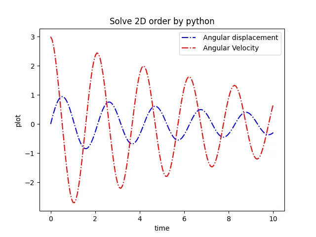
Animation video link

https://youtu.be/buSfY7cXjGs