Week 3 - Solving second order ODEs

Aim:

To write a program that solves the following ODE. This ODE represents the equation of motion of a simple pendulum.

Procedure:

Damping:

Damping is an influence within or upon an oscillatory system that has the effect of reducing or preventing its oscillation. In physical systems, damping is produced by processes that dissipate the energy stored in the oscillation.

Types of damping:

Viscous damping

Imagine dropping an object. While that object is falling through the air, the only force acting against it is the air resistance. If you dropped the object into water or oil, it would begin slowing down at a higher rate until eventually stopping. This is the concept of viscous drag. Applying this concept to everyday life explains the physics of automatic doors or anti-slam doors.

Damping in electric system:

Electrical systems that operate with alternative current(AC) use resistors to damp the electrical current, since they are periodic. Dimmer switches or volume knobs are examples of damping in an electrical system.

Magnetic damping:

Kinetic energy that causes oscillations is dissipated as heat by electric eddy currents which are induced by passing through a magnet's poles, either by a coil or aluminum plate. In other words, the resistance caused by magnetic forces slows a system down. An example of this concept being applied to the real world is the brakes on roller coasters.

The below formula used in the program for solving the ODE.

Program:

import numpy as np
from scipy.integrate import odeint
import matplotlib.pyplot as plt
import math

#Function that returns dz/dt
def model(theta,t,b,g,l,m):
	theta1 = theta[0]
	theta2 = theta[1]
	dtheta1_dt = theta2
	dtheta2_dt = -(b/m)*theta2-(g/l)*math.sin(theta1)
	dtheta_dt = [dtheta1_dt,dtheta2_dt]
	return dtheta_dt

b = 0.05
g = 9.81
l = 1
m = 0.1

#Initial Condition
theta_0 = [0,5]

#Time point
t = np.linspace(0,20,200)
#Solve ODE
theta = odeint(model, theta_0, t, args=(b,g,l,m))

plt.plot(t,theta[:,0],'b-')
plt.plot(t,theta[:,1],'r--')
plt.xlabel('time')
plt.ylabel('plot')
plt.show()
ct = 1

#Creating animation for simple pendulum
for t in theta[:,0]:
	x0 = 0
	y0 = 0
	x1 = l*math.sin(t)
	y1 = -l*math.cos(t)
	filename = str(ct)+'.png'
	ct = ct+1

	plt.figure()
	plt.plot([-0.2,0.2],[0,0],linewidth=5)
	plt.plot([x0,x1],[y0,y1],linewidth=3,color='b')
	plt.plot(x0,y0,'o',markersize=5)
	plt.plot(x1,y1,'o',markersize=30,color='green')
	plt.xlim([-1.5,1])
	plt.ylim([-1.5,1])
	plt.title('Motion of simple pendulum')
	plt.savefig(filename)

Code Explanation:

• To solve the ODE, from scipy.intergrate import odeint and numpy.
• Breaking down the second order into first order so that it can be solved quickly.
• The initial angular displacement and velocity were defined by the theta_0 array. The time input(0 to 20 secs) and was split in 200 parts using linspace command for plotting the curve.
• A function was defined for calculating the angular displacement and velocity at different time intervals. The second-order differential equation defining the motion of pendulum ( `(d^2theta)/(dt^2) + (b/m)*(d theta)/dt +(g/l)sin theta=0`) was split into 2 single order differential equations (`(d theta_1)/ (dt)=theta_2`) and (`(d theta_2)/(dt) = -(b/m)*theta2 - (g/l)*sintheta1`) and defined within the function. odeint was used to solve this differential equation with given input parameters.
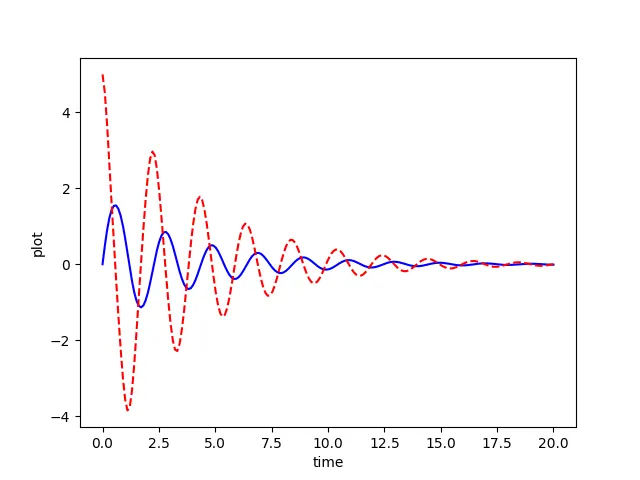
• For the displacement and velocity grapg is plotted.
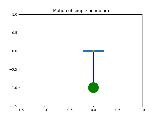
• For the animation multiple image has been captured and combined together with the imagemagick.

Graph:

The movement of the pendulum with damping.

Animation of simple pendulum:

Uploaded youtube link:

https://youtu.be/EJp6R5SToIc

Result:

The conclusion shows that the displacement and velocity i.e., the motion of the pendulum goes on decrease with respect to the damping force.