Week 3 - Solving second order ODEs

Problem Statement: Solving 2nd Order ODEs for a Simple Pendulum Probem

Objective:

To solve a 2nd order ODE problem of a simple pendulum and simulate its kinematics in MATLAB

Explanation to the code:

• The 2nd order Differetial equation that gives the angular postion of the ball with respect to time is
  `(d^2 (theta))/dt^2+(b/m)(d theta)/dt+(g/l)sin(theta)=0`
• The values such as length of pendulum,mass of the bob ,damping coefficient and gravitational constant were given as inputs.
• The time period of oscillation was defined using the 'linspace' function for 20s by giving a resolution of 200 time intervals.
• The original ODE was simplified into two first order differential equations, and made into a a matrix so that MATLAB variables can be defined and 'ode45' function could be used.
  `[[(d(theta_1))/dt ],[(d(theta_2))/dt ]]=[[theta_2],[(d(theta_2))/dt+(g/m)theta_2+(g/l)sin(theta_1)]]`
• The angular displacement obtained were then plotted to get the animation.

Link to the video:

https://www.youtube.com/watch?v=pevJTA3Qf1I

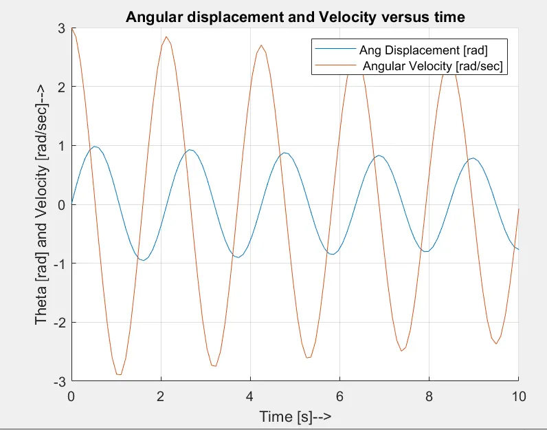
Output plot for Figure 1:

Main Code:

%Pendulum Simulation
close all
clear all 
clc 

%Input parameters
l=1;         %length of the pendulum [m]
m=1;         %mass of the Bob [kg]
b=0.05;      %Damping coefficient [dimensionless]
g=9.8;       %gravitational Constant [m s^-2]

%Initial Conditions
theta_initial=[0;3];

%time span of 20s with 100 intervals 
t_span=linspace(0,20,100);

%solving the ODE equation using 'ode45' function
[t,results]=ode45(@(t,theta) ode_function(t,theta,b,g,l,m),t_span,theta_initial);

%plotting the results 
figure(1)
hold on 
plot(t_span,results(:,1)) %extracting first column of angular displacement.
plot(t_span,results(:,2)) %extracting the second column of speed.
grid on
title('Angular displacement and Velocity versus time')
xlabel('Time [s]-->')
ylabel('Theta [rad] and Velocity [rad/sec]-->')
legend('Ang Displacement [rad]',' Angular Velocity [rad/sec]')
x0=0;
y0=0;
ct=1;
theta=results(:,1);

%plotting the animation of simple pendulum.
%plotting in the 3rd and 4th quadrant
figure(2)
for i=1:length(theta)
    x=l*cos(theta(i)+(3*pi/2));
    y=l*sin(theta(i)+(3*pi/2));
    
    plot([x0 x],[y0 y],'linewidth',1,'color','k')
    hold on
    xline(0,'--','Reference')
    plot(x,y,'o','color','r','MarkerSize',20,'MarkerFaceColor','red','MarkerEdgeColor','k')
    text(x+(x*0.1),y+(y*0.1),'Bob')
    hold off
    axis([-1 1 -1.2 0])
    title('Simple Pendulum Motion')
    pause(0.1)
    M(ct)=getframe(gcf);
    ct=ct+1;
end
movie(M);
videofile=VideoWriter('Simple Pendulum Motion.avi','Uncompressed AVI');
videofile.FrameRate=8;      %Determining Frame rate of the video
open(videofile);            %opening a movie file
writeVideo(videofile,M);    %Writing the frames to it
close(videofile);           %closing the video file 

The Corresponding ODE function used is-'ode_function' the code for which is down:

function [dtheta_dt]=ode_function(t,theta,b,g,l,m)
    theta1=theta(1); %defining theta1 
    theta2=theta(2); %defining theta2
    
    dtheta1_dt=theta2;
    dtheta2_dt=-(b/m)*theta2-(g/l)*sin(theta1);
    dtheta_dt=[dtheta1_dt;dtheta2_dt];
end