Week 3 - Solving second order ODEs

AIM:

To animate the motion of the pendulum bob by solving second order ode.

OBJECTIVE:

Animation of the pendulum.

GOVERNING EQUATION:

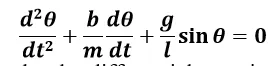
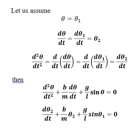
Let’s convert the above second-order differential equation into a first-order differential equation.

FUCTION CODE:

1. function [dtheta_dt] = ode_fun(t,theta,b,g,l,m)
2. theta1 = theta(1)
3. theta2 = theta(2)
4. dtheta1_dt = theta2
5. dtheta2_dt = -(b/m)*theta2-(g/l)*sin(theta1)
6. dtheta_dt = [dtheta1_dt;dtheta2_dt]
7. end

The above governing equation is converted into a function

MAIN CODE:

1. clear all
2. close all
3. clc
4. %initial and boundary conditions
5. b = 0.1; %damping coefficient kg/s
6. g = 9.81; %acceleration due to gravity m/s
7. l = 1; %length of the cord in m
8. m = 0.1; %mass of the bob in kg
9. theta_0 = [0;5];
10. t_span = linspace(0,10,100);
12. % solver
13. [t,results] = ode45(@(t,theta)ode_fun(t,theta,b,g,l,m),t_span,theta_0);
15. %ploting
16. figure(1)
17. plot(t,results(:,1))
18. hold on
19. plot(t,results(:,2))
20. hold off
21. ylabel('angular displacement')
22. xlabel('time')
24. %animating using the data
25. ct = 1;
26. for i = 1:length(results(:,1))
27. theta = results(i,1);
28. x0 = 0;
29. y0 = 0;
31. x1 = 1*sin(theta);
32. y1 = -1*cos(theta);
34. %plotting the bob
35. figure(2)
36. plot([-1,1],[0,0],"b-","linewidth",5)
37. hold on
38. plot([x0,x1],[y0,y1],"b-","linewidth",2)
39. axis([-2 2 -2 2])
40. plot(x1,y1,"o","MarkerSize",20,"MarkerFaceColor","r")
41. hold off
42. grid on
43. axis([-2 2 -2 2])
44. pause(0.01)
45. M(ct) = getframe(gcf);
46. ct = ct+1;
47. end
49. %making plots into video
50. Video = VideoWriter("pedulum_animation");
52. open(Video)
53. writeVideo(Video,M)
54. close(Video)

EXPLAINING THE CODE:

1. Load the initial conditions.
2. Ode45 is a solver that uses range kutta method to solve first order differential equation. The initial conditions and boundary conditions are given to the solver. The function that is crated from the first order differential equation is also mentioned.
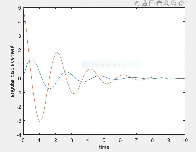
3. We plot the results with respective to t.
4. Now to animate the pendulum we have to plot the every position the bob has been to do that we use for loop. The values of the results are used as inputs for the loop and the position of the bob is determined and plotted. We save the plots in a file using getframe function.
5. Videowriter function is used to video data from an array.
6. writeVideo is used to write video into a file.

ERRORS:

There are no major errors occurred.

RESULTS:

The animation is complete and the link is here

https://youtu.be/K0_yC6o2aek

the plot figure 1