Week 3 - Solving second order ODEs

Objective

In this project, it is aimed to write the coding of the oscillation movement of a 1 kg hanging mass with a damping value of 0.05 at a speed of 3 rad / s for 20 seconds from its initial position in equilibrium.

Problem Statement

The equation of simple damped pendulum motion with initial conditions of the system can be expressed by 2nd order ordinary differential equations. A code is required to solve the equation set for the 2nd order ordinary differential.

Solution Procedure

math, matplotlib, numpy and scipy libraries are used in this code. Then, conversion is done for two ordinary differential systems to be used in the solution of the equation of motion, and the sets of equations expressing these differentials are printed in the function as the solution vector. This function is then solved for the targeted initial conditions with the scipy integrator.

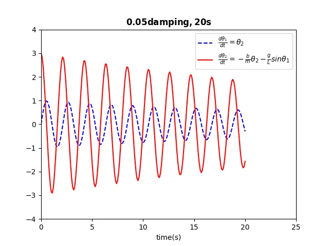
The graphs contain the first ordinary differential, which will give the time-dependent variation of the angle, and the second ordinary differential results, which will show the time-dependent variation of the angular velocity. The picture is recorded and animated for the temporal coordinates of the pendulum moving point.

Results and Discussion

The graph below shows the variation of angle and angular velocity with time in the pendulum system. Where the angle is maximum, the velocity is zero where the velocity is maximum.

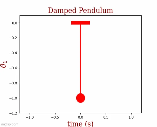
and the animation of the pendulum system obtained with the second order ordinary differential solution is as follows.

Code

"""
SIMPLE DAMPED PENDULUM SYSTEM by 2nd order ODE
by omerfarukgumus

"""

import numpy as np 
from scipy.integrate import odeint 
import math
import matplotlib.pyplot	as plt 


# function for problem

def simple_pendulum(theta,time,b,g,l,m):

	diff_1=theta[0]
	diff_2=theta[1]
	theta1_dt=diff_2
	theta2_dt=-(b/m)*diff_2-(g/L)*math.sin(diff_1)
	sol_vector=[theta1_dt,theta2_dt]
	return	sol_vector


b=0.05		#Damping coefficient
g=9.81		#Gravitation in m/s^2
L=1			#length in meter
m=1		#mass in kg


#INITIAL CONDITIONS

theta_initial=[0,3]

#ELAPSED TIME
time=np.arange(0,20.1,0.1)
print(time)

#SOLVING ODE

theta=odeint(simple_pendulum,theta_initial,time,args=(b,g,L,m))


#PLOTTING 
plt.figure(1)
plt.plot(time,theta[:,0],'b--',label=r'$\mathit{\frac{d\theta_1}{dt}=\theta_2}$')
plt.plot(time,theta[:,1],'r-',label=r'$\mathit{\frac{d\theta_2}{dt}=-\frac{b}{m}\theta_2-\frac{g}{L}sin\theta_1}$')
plt.legend(loc='best')
plt.xlabel('time(s)',fontsize=10)
#plt.ylabel(r'$/theta_1')
plt.xlim([0,25])
plt.ylim([-4,4])
plt.title(r'$\mathbf{0.05 damping, 20s}$',fontsize=12)
plt.show()



#PLOTTING AND SAVING SEQUENTIALLY TO CREATE AN ANIMATION

x1=[]
y1=[]
ct=0
font = {'family' : 'serif',
        'color'  : 'darkred',
        'weight' : 'normal',
        'size'   : 20
        }

for t in theta[:,0]:
	x0=0
	y0=0
	x1=(L*math.sin(t))
	y1=-(L*math.cos(t))
	ct=ct+1
	filename='pendulum%03d' %ct
	plt.figure()
	plt.plot([-0.15,0.15],[0,0],'r',linewidth=10)	#fixed part of the pendulum system
	plt.plot([x0,x1],[y0,y1], 'r' ,linewidth=3)		#Pendulum bar
	plt.plot(x1,y1,'r',marker='o',markersize=25)	#mass of the pendulum system
	plt.xlim([-1.2,1.2])
	plt.ylim([-1.2,0.1])
	plt.title('Damped Pendulum', fontdict=font)
	plt.xlabel('time (s)', fontdict=font)
	plt.ylabel(r'$\theta_1$', fontdict=font)
	plt.savefig(filename)