Solving second order ODEs using Matlab

Aim: Write a program that solves the second order which represents the equation of motion of a simple pendulum with damping.

Introduction :

what is second order ode's ?

A second order ordinary differential equation is an ordinary differential equation in which any derivates with respect to the independent variable have order no greater than 2.The general second order ODE can be written as:

x"(t) = F(t, x(t), x'(t))

In Engineering problems, ODE is used to describe the transient behavior of a system. A simple example is a pendulumThe way the pendulum moves depends on the Newtons second law. When this law is written down, we get a second order Ordinary Differential Equation that describes the position of the "ball" w.r.t time.

Pendulum, body suspended from a fixed point so that it can swing back and forth under the influence of gravity. Pendulums are used to regulate the movement of clocks because the interval of time for each complete oscillation, called the period, is constant. The formula for the period T of a pendulum is T = 2π Square root of√^L/_g, where L is the length of the pendulum and g is the acceleration due to gravity.

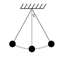
Here we use input parameters are:

Length=1 metre,

mass=1 kg,

Damping Co-efficient(b)=0.05.

g=9.81 m/s2.

And we simulate the motion between 0-20 sec, for angular displacement=0,angular velocity=3 rad/sec at time t=0.

The complete code

close all
clc

%input parameters for the model
b = 0.05;
m = 1;
l = 1;
g = 9.81;

%angular displacemnt and angular velocity at time=0sec
theta_0 =[0;3];

%Simulate the motion between 0-20 sec
t_span = linspace(0,20,100);

%solving second order ode using ode45
[t , results] = ode45(@(t,theta) ode_function(t,theta,b,g,l,m),t_span,theta_0);

k = results;
displacement = k(:,1);
velocity = k(:,2);

%plot the graph between time vs angular displacement
figure(1)
plot(t,displacement,'linewidth',1,'color','b')
title('time vs displacement')
xlabel('Time')
ylabel('Angular Displacement')

%
%plot the graph between time vs angular velocity
figure(2)
plot(t,velocity,'linewidth',1,'color','r')
title('time vs angularvelocity')
xlabel('Time')
ylabel('Angular velocity')

%Animating simple pendulum motion 
ct = 1;
for i=1:length(t)
    x0 = 0 ;
    y0 = 0 ;
    x = l*cos((pi/2)-results(i));
    y = -l*sin((pi/2)-results(i));
    
    %plot of pendulum line from origin
    figure(3)
    plot([-1,1],[0,0],'linewidth',5)
    hold on
    plot([x0 x],[y0 y],'linewidth',3)
    hold on
   
    %plot of pendulum location of pendulum at x,y
    plot(x,y,'o','markersize',20,'MarkerFaceColor','g')
    axis([-1.5 1.5 -1.5 1])
    grid on
    xlabel('X-axis')
    ylabel('Y-axis')
    title('Motion of Simple Pendulum')
    pause(0.005)
    hold off
    
    M(ct) = getframe(gcf)
    ct = ct+1
end

%animation
movie(M)
videofile = VideoWriter('pendulum8.avi','Uncompressed AVI')
open(videofile)
writeVideo(videofile,M)
close(videofile)

The code for Function

function [dtheta_dt] = ode_function(t,theta,b,g,l,m)
    
    theta1 = theta(1);
    theta2 = theta(2);
    dtheta1_dt = theta2;
    dtheta2_dt = -(b/m)*theta2 - (g/l)*sin(theta1);
    dtheta_dt = [dtheta1_dt;dtheta2_dt];
    
end

Explanation of code step wise

clc
clear all
close all

• This clears your workspace, clears command window and closes all figures.

%input parameters for the model
b = 0.05;
m = 1;
l = 1;
g = 9.81;

• In the above code
• g = gravity in m/s2,
• L = length of the pendulum in m,
• m = mass of the ball in kg,
• b=damping coefficient.

%angular displacemnt and angular velocity at time=0sec
theta_0 =[0;3];

%Simulate the motion between 0-20 sec
t_span = linspace(0,20,100);

• In the above code theta_0 = [0;3] are the angular displacement and angular velocity at time = 0sec and t_span is the time where we Simulate the motion between 0-20 sec at 100 intervals.

function [dtheta_dt] = ode_function(t,theta,b,g,l,m)
    
    theta1 = theta(1);
    theta2 = theta(2);
    dtheta1_dt = theta2;
    dtheta2_dt = -(b/m)*theta2 - (g/l)*sin(theta1);
    dtheta_dt = [dtheta1_dt;dtheta2_dt];
    
end

• The above code is function of following ODE, which represents the equation of motion of a simple pendulum with damping

ode45

• Solve nonstiff differential equations — medium order method.An ordinary differential equation (ODE) is an equation that involves some ordinary derivatives (as opposed to partial derivatives) of a function. Often, our goal is to solve an ODE, i.e., determine what function or functions satisfy the equation.

%plot the graph between time vs angular displacement
figure(1)
plot(t,displacement,'linewidth',1,'color','b')
title('time vs displacement')
xlabel('Time')
ylabel('Angular Displacement')

%
%plot the graph between time vs angular velocity
figure(2)
plot(t,velocity,'linewidth',1,'color','r')
title('time vs angularvelocity')
xlabel('Time')
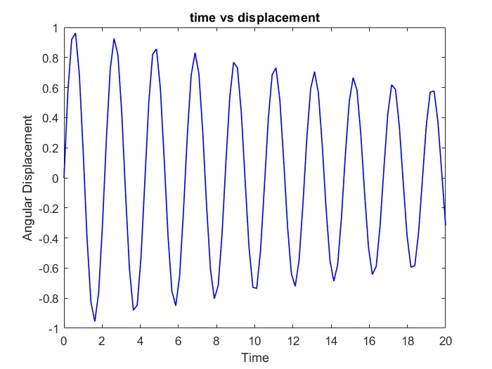
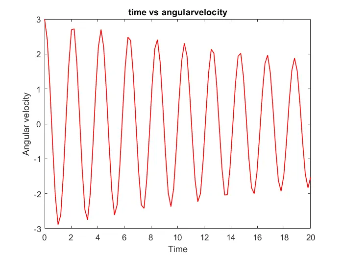
ylabel('Angular velocity')

• The above code is to plot the graph between time vs angular displacement and angular velocity.The images of the plot are as shown below.

%Animating simple pendulum motion 
ct = 1;
for i=1:length(t)
    x0 = 0 ;
    y0 = 0 ;
    x = l*cos((pi/2)-results(i));
    y = -l*sin((pi/2)-results(i));
    
    %plot of pendulum line from origin
    figure(3)
    plot([-1,1],[0,0],'linewidth',5)
    hold on
    plot([x0 x],[y0 y],'linewidth',3)
    hold on
   
    %plot of pendulum location of pendulum at x,y
    plot(x,y,'o','markersize',20,'MarkerFaceColor','g')
    axis([-1.5 1.5 -1.5 1])
    grid on
    xlabel('X-axis')
    ylabel('Y-axis')
    title('Motion of Simple Pendulum')
    pause(0.005)
    hold off
    
    M(ct) = getframe(gcf)
    ct = ct+1
end

%animation
movie(M)
videofile = VideoWriter('pendulum8.avi','Uncompressed AVI')
open(videofile)
writeVideo(videofile,M)
close(videofile)

• In the above code we use for loop to iterate the location of pendulum for every value in t and then we made an animation.
• A "For" Loop is used to repeat a specific block of code a known number of times.
• we wanted to plot the graph for every interval of [x y] and [x y].
• VideoWriter command helps us in Create object to write video files we store the video created in the variablewith the name of videofile.
• open command helps to opens the specified file or variable in the appropriate application.
• writeVideofile writes data from an array to the video file associated with M.
• After running the whole code after our videofile is created and stored.

The Animation of video file is in the below: