Week 3 - Solving second order ODEs
Solving second order ODEs
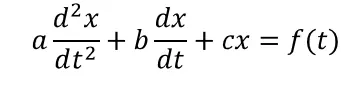
Aim: to write a program that solves the following ODE. This ODE represents the equation of motion of a simple pendulum with damping.
Introduction: . For an understanding of simple harmonic motion it is sufficient to investigate the solution of differential equations with constant coefficients. [1]
A simple pendulum consists of a particle of mass attached to one end of a light inextensible string of length where the other end of the string is attached to a fixed point. The particle when at rest hangs vertically below the fixed point. The particle and string when displaced from the equilibrium position oscillate in a circular arc in the same vertical plane.
`(d^2theta)/(d t^2) + b/m* (d theta)/(d t) + g/L* Sin theta = 0`
In the above equation,
g = gravity in m/s2,
L = length of the pendulum in m,
m = mass of the ball in kg,
b=damping coefficient.
Input data.
L=1 metre,
m=1 kg,
b=0.05.
g=9.81 m/s2.
Simulate the motion between 0-20 sec, for angular displacement=0,angular velocity=3 rad/sec at time t=0.
`(d^2theta)/(d t^2) + b/m* (d theta)/(d t) + g/L* Sin theta = 0` eq 0.1
This is a 2nd order differential equation. So So do the transformation.
` theta = theta_1`
`(d theta)/(d t) = (d theta_1)/(d t) = theta_2` ............eq 1
`(d^2theta)/(d t^2) = (d^2theta_1)/(d t^2) = d/dt( (d theta_1)/(d t))= d/dt (theta_2)` .......eq2
Substitute 1 nad 2 in 0.1
`(d^2theta_1)/(d t^2) + b/m* (d theta_1)/(d t) + g/L* Sin theta_1 = 0`
`(d theta_2)/(d t) + b/m* theta_2 + g/L* Sin theta_1 = 0`
`(d theta_1)/(d t) = theta_2`
`(d theta_2)/(d t) = - b/m* theta_2 - g/L* Sin theta_1`
So Write it in solution vector form
`d/dt[[theta_1],[theta_2]] = [[theta_2],[- b/m* theta_2 - g/L* Sin theta_1]]`
ode45
Solve a set of non-stiff Ordinary Differential Equations (non-stiff ODEs) with the well known explicit Dormand-Prince method of order 4.
fun is a function handle, inline function, or string containing the name of the function that defines the ODE: y' = f(t,y). The function must accept two inputs where the first is time t and the second is a column vector of unknowns y.
The function typically returns two outputs. Variable t is a column vector and contains the times where the solution was found. The output y is a matrix in which each column refers to a different unknown of the problem and each row corresponds to a time in t.[2]
[t,results] = ode45(@(t,theta) ode_func(t,theta,b,g,L,m),t_span, theta_0);
Calling function in side ode45 for diffrent values of time t_span and intial condition
@(t, theta) meant ode_func is the function of t and theta, ode_func(t, theta,b,g,L,m) is how Ode is defining
t_span how much time we have read reasults
theta_0 is reads the vaules of displacement and angular velocity for every value of t_span
we will get angular velocity, displacement at time 't'
Function:
function [dtheta_dt] = ode_func(t,theta,b,g,L,m)    %  dtheta_dt is the function of t,theta,b,g,L,m
  theta1 = theta(1);                                % theta1 is the first value of theta_0 which is displacement
  theta2 = theta(2);                                % theta2 is the 2nd value of theta_0 which is velocity.

  % from the equations we have
  dtheta1_dt = theta2;
  dtheta2_dt = -(b/m)*theta2 - (g/L)*sin(theta1);
  dtheta_dt = [dtheta1_dt ; dtheta2_dt];
  end
Program:
% write a program that solves the following ODE. This ODE represents the equation of motion of a simple pendulum with damping.

close all
clear all
clc

% Input data
L=1;             % length of the pendulum in m,
m=1;             % mass of the ball in kg,
b=0.05;          % damping coefficient.
g=9.81;          % gravity in m/s2,

% Initial Condition

theta_0 = [0;3];   % we have 2 first order diffrencial equations , one id for displacement and other one is for velocity
    % So here initial displacement is 0 and initial velocity is 3 m/s

% time between 0-20 sec,
t_span = linspace(0,20,250);

% Calling function in side ode45 for diffrent values of time t_span and intial condition
%@(t, theta) meant ode_func is the  function of t and theta,
% ode_func(t, theta,b,g,L,m) is how Ode is defining
% t_span how much time we have read reasults
% theta_0 is reads the vaules of displacement and angular velocity for every value of t_span
% we will get angular velocity, displacement at time 't'

[t,results] = ode45(@(t,theta) ode_func(t,theta,b,g,L,m),t_span, theta_0);

% Plots
figure(1)
plot(t,results(:,1),'linewidth',1.5)
hold on
plot(t,results(:,2),'linewidth',1.5)
grid on
xlabel('time in s')
ylabel('angular displacement in theta and Velocity in m/s')
legend('angular displacement',' Velocity')


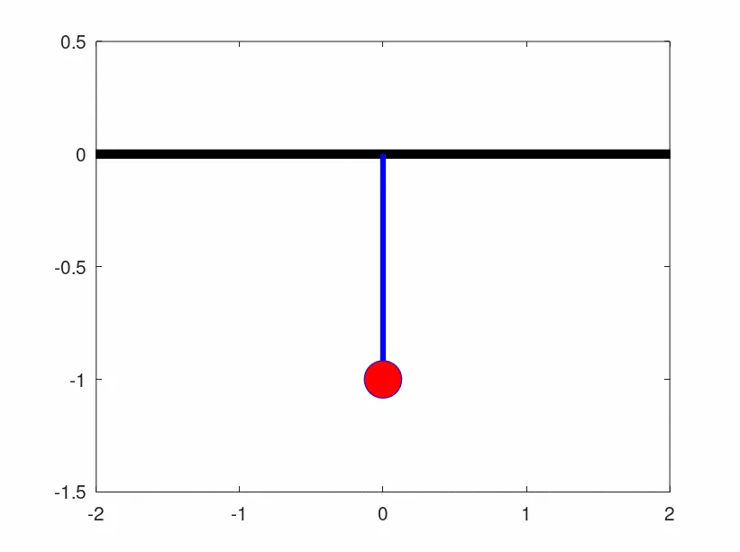
%  pendulum animation
ct = 1;
for i = 1 : length(results(:,1)); % where i value varies from 1 to length of results in first column i e angular displacement
 % consider for fixed end of pendulum is at x0 and y0
 x0 = 0;
 y0 = 0;

 % for the coordinates x1 and y1, which are varing wrt angular displacement,
 % x1 = length of string * sind(theta) and  y1 = length of string * cosd(theta)

 x1 = L*sin(results(i,1));       % coordinate value at theta1 in x axis
 y1 = -(L*cos(results(i,1)));      % coordinate value at theta1 in y axis

 % plots
 figure(3)
 plot([-5 5],[0 0],'color','k' ,'linewidth',5 );
 axis([-2 2 -1.5 0.5])
 hold on
 plot([x0,x1],[y0,y1],'linewidth',3,'color','b');
 plot(x1,y1,'o','markersize', 20, 'markerfacecolor', 'r','color','b');
 pause(0.03)
 hold off

%Create Gif
printf('Creating GIF- Progress... %d', ct)
ct = ct + 1;
img = print ('-RGBImage');
imwrite(img, 'animation.gif', 'DelayTime', .005, 'Compression', 'bzip', 'WriteMode', 'Append');

end
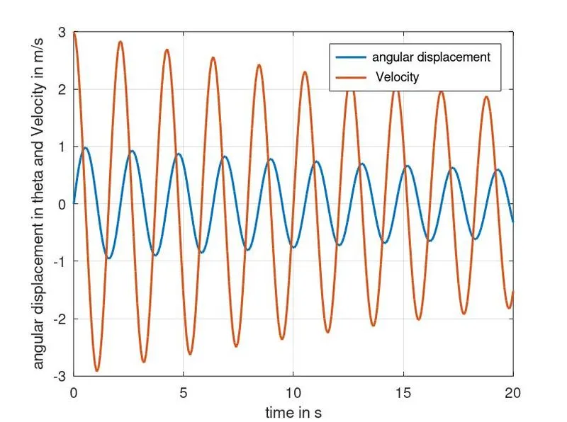
Results: a program that solves the following ODE. This ODE represents the equation of motion of a simple pendulum with damping is done for time span 0-20 sec, for angular displacement=0,angular velocity=3 rad/sec at time t=0.
1.from the plot we can say that the angular displacement at time t os zero and angular velocity is maximum 3 rad/sec. as time increases the angular velocity and angular displacement are going reduceses. this is due to damping coefficient and gravity.
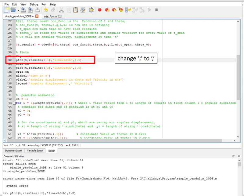
errors
Referance:
[1]. http://www.casaxps.com/help_manual/mathematics/Mechanics3_rev12.pdf
[2]. https://octave.sourceforge.io/octave/function/ode45.html