Week 3 - Solving second order ODEs

AIM:

To write a program that solves the following ODE and to create an animation video using MATLAB.

OBJECTIVES:

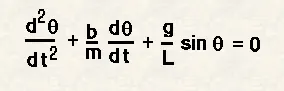
Where,

b = 0.05

m = 1kg

g = 9.81 m/s²

L = 1m

Angular Displacement = 0

Angular Velocity = 3 rad/sec at time t = 0

THEORY:

In mathematics, an ordinary differential equation (ODE) is a differential equation containing one or more functions of one independent variable and the derivatives of those functions.

So here we have a Second order ODE,

Where,

b = damping coefficient

m = mass of the ball in kg

g = gravity in m/s2

L = length of the pendulum in m.

A Couple of examples for a second order ODE are Simple Pendulum and Spring Damper.

Since we have given a second order ODE, we break it down as a single order ODE to solve it. So let’s say that,

θ = θ1

Therefore,

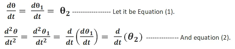
Now getting back to the given ODE,

Substituting θ₁ to θ,

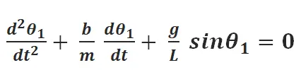
Then,

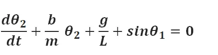
So here we’ve created two ODEs,

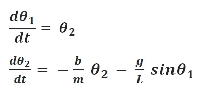
PROGRAM:

clear all 
close all
clc

b = 0.05;
g = 9.81;
l = 1;
m =0.1;
t= 0;
%Initial condition
theta_0 = [0;3];

%Time points
t_span = linspace(0,20,500);

%Solve ODE
[t,results] = ode45(@(t,theta) ode_func(t,theta,b,g,l,m),t_span,theta_0);
 
plot(t,results(:,1))
hold on
plot(t,results(:,2))
xlabel('plot')
ylabel('time')

Starting with clearing commands, clear all, close all and clc.

Giving the values for inputs b,g,l,m and t as shown.

So we've break down the second order ODE into two first order ODEs. Which brings us two initial conditions, Displacement and Velocity.

And next is solving the ODE, starting with "ode45"; an in-built solved in MATLAB. Then considering "(t,theta)" as the main inputs and so we are saying that our ODE is function of "(t,theta)". Next we define our function and after that we provide the Time array and Initial conditions.

Then comes the plot command which helps to plot the graph. Then labeling the graph helps us conclude.

function [dtheta_dt]= ode_func(t,theta,b,g,l,m)

theta1 = theta(1);
theta2 = theta(2);
dtheta1_dt = theta2;
dtheta2_dt = -(b/m)*theta2 - (g/l)*sin(theta1);
dtheta_dt = [dtheta1_dt;dtheta2_dt];

end

Then we provide theta values to be considered.

And we are executing the two ODEs to solve the function.

So by doing this we get a graph of pendulum oscillation in certain conditions given. Still it is not complete without an animation video.

Now the code for animation.

clear all 
close all
clc

b = 0.05;
g = 9.81;
l = 1;
m =0.1;
t= 0;
%Initial condition
theta_0 = [0;3];

%Time points
t_span = linspace(0,20,500);

%Solve ODE
[t,results] = ode45(@(t,theta) ode_func(t,theta,b,g,l,m),t_span,theta_0);
 
% plot(t,results(:,1))
% hold on
% plot(t,results(:,2))
% xlabel('plot')
% ylabel('time')

 ct=1;
 for i = 1:length(t_span);
   THETAl(i)= results(i,1);

  x0=0;
  y0 = 0;

 y1 = -l*cos(THETAl(i));
 x1=  l*sin(THETAl(i));
 
 
 %figure (ct)

   plot ([x0 x1],[y0 y1],'linewidth',3);
   axis([-2 2 -1.5 0.5]);
  hold on
   plot(x1,y1,'marker','o','markersize',15,'markerfacecolor','r');

    hold off
   M(ct)= getframe(gcf); 
   ct=ct+1;

 end

movie(M);
videofile=VideoWriter('pendulum motion3.avi','uncompressed avi');
open(videofile);
writeVideo(videofile,M);
close(videofile);

We will start from the counter command after the ploting commands.

And add forloop command to make loop for length of time array.

Then providing the needed length and dimensions of pendulum.

Then giving out the axis from where the pendulum must start and stop etc. With the required linewidth, markersize, etc.

Next giving the "getframe" command. And ending the foorloop.

Now we are creating a movie of this plot in required folder and path.

At last we are closing it.

Video link:

https://youtu.be/jBMZuK1XrK4

RESULT:

Solved the following ODE and created an animation video using MATLAB.