Week 3 - Solving second order ODEs
OJECTIVES :- To solve second order ODEs in MATLAB by giving a simple example is a pendulum.
PROBLEM STATEMENT :-
In Engineering, ODE is used to describe the transient behaviour of a system. A simple example is a pendulum.
The way pendulum moves depends on the Newtons second law. When this law is written dawn, we get a a second order ODE that describe the position of the ball w.r.to time.
Similarly, there are hundreds of ODEs that describes key phenomenon and if we have the ability to solve these equations then we will be able to simulate any of these systems.
Our objective is to write a program that solves the following ODE. This ODE represents the equation of motion of a simple pendulum with damping.
In the above equation,
g = acceleration due to gravity in m/s^2,
L = length of the pendulum in m,
m = mass of the ball in kg,
b = damping coefficient,
Write a program in Matlab that will simulate the pendulum motion. Use,
L = 1m,
m = 1kg,
b = 0.05,
g = 9.81 m/s^2
Simulate the motion between 0-20 sec, for angular displacement = 0, angular velocity = 3 rad/sec at time, t=0.
Whe we do this we will get the position of the pendulum as a function of time. Use this information to animate the motion of the pendulum.
2. Submit a report that has the following contents-
- Step wise explaination of our code
- Error faced while programming
- How have we overcome those errors
- Screenshot showing a error thrown in command window.
THEORY & INTRODUCTIONS :-
Nonlinear Pendulum
Differential Equation of Oscillations
Pendulum is an ideal model in which the material point of mass m is suspended on a weightless and inextensible string of length L. In this system, there are periodic oscillations, which can be regarded as a rotation of the pendulum about the axis O (Figure 1).
Dynamics of rotational motion is described by the differential equation
ε=d2αdt2=MI,
where ε is the angular acceleration, M is the moment of the force that causes the rotation, I is the moment of inertia about the axis of rotation.
In our case, the torque is determined by the projection of the force of gravity on the tangential direction, that is
M=−mgLsinα.
The minus sign indicates that at a positive angle of rotation α (counterclockwise), the torque of the forces causes rotation in the opposite direction.
The moment of inertia of the pendulum is given by
I=mL2.
Then the dynamics equation takes the form:
d2αdt2=−mgLsinαmL2=−gsinαL,⇒d2αdt2+gLsinα=0.
In the case of small oscillations, one can set sinα≈α. As a result, we have a linear differential equation
d2αdt2+gLα=0ord2αdt2+ω2α=0,
where ω=√gL is the angular frequency of oscillation.
The period of small oscillations is described by the well-known formula
T=2πω=2π√Lg.
However, with increasing amplitude, the linear equation ceases to be valid. In this case, the correct description of the oscillating system implies solving the original nonlinear differential equation.
Period of Oscillation of a Nonlinear Pendulum
Suppose that the pendulum is described by the nonlinear second order differential equation
d2αdt2+gLsinα=0.
We consider the oscillations under the following initial conditions
α(t=0)=α0,dαdt(t=0)=0.
The angle α0 is the amplitude of oscillation.
The order of the equation can be reduced, if we find a suitable integrating factor. Multiply this equation by the integrating factor dαdt. This leads to the equation
d2αdt2dαdt+gLsinαdαdt=0,⇒ddt[12(dαdt)2−gLcosα]=0.
After integration we obtain the first order differential equation:
(dαdt)2−2gLcosα=C.
Given the initial conditions, we find the constant C:
C=−2gLcosα0.
Then the equation becomes:
(dαdt)2=2gL(cosα−cosα0).
Next, we apply the double angle identity
cosα=1−2sin2α2,
which leads to the following differential equation:
(dαdt)2=4gL⋅(sin2α02−sin2α2),⇒dαdt=2√gL⋅√sin2α02−sin2α2.
Integrating this equation, we obtain
∫d(α2)√sin2α02−sin2α2=√gL∫dt.
We denote sinα02=k and introduce the new variable θ instead of the angle α:
sinα2=sinα02sinθ=ksinθ.
Then
d(sinα2)=cosα2d(α2)=√1−sin2α2d(α2)=√1−k2sin2θd(α2)=kcosθdθ.
It follows that
d(α2)=kcosθdθ√1−k2sin2θ.
In the new notation, our equation can be written as
∫kcosθdθ√1−k2sin2θkcosθ=√gL∫dt,⇒∫dθ√1−k2sin2θ=√gL∫dt.
Next, we discuss the limits of integration. The passage of the arc from the lowest point α=0 to the maximum deviation α=α0 corresponds to a quarter of the oscillation period T4. It follows from the relationship between the angles α and θ that sinθ=1 or θ=π2 at α=α0. Therefore, we obtain the following expression for the period of oscillation of the pendulum:
√gLT4=π2∫0dθ√1−k2sin2θorT=4√Lg⋅π2∫0dθ√1−k2sin2θ.
The integral on the right cannot be expressed in terms of elementary functions. It is the so-called complete elliptic integral of the 1st kind:
K(k)=π2∫0dθ√1−k2sin2θ.
The function K(k) is computed in most mathematical packages. Its graph is shown below in Figure 2.
The function K(k) can also be represented as a power series:
K(k)=π2{1+(12)2k2+(1⋅32⋅4)2k4+(1⋅3⋅52⋅4⋅6)2k6+…+[(2n−1)!!(2n)!!]2k2n+…},
where the double factorials (2n−1)!! and (2n)!! denote the product, respectively, of odd and even natural numbers.
Note that if we restrict ourselves to the zero term of the expansion, assuming that K(k)≈π2, we obtain the known formula for the period of small oscillations:
T0=4√LgK(k)≈4√Lgπ2=2π√Lg.
Further terms of the series for n≥1 are just allow to consider the anharmonicity of the oscillations of the pendulum and the nonlinear dependence of the period T on the oscillation amplitude α0.
Que. 1) What is ode45 function in Matlab ?
Ans. :- ode45 is usually the function of choice among the ODE solvers. It compares methods of orders four and five to estimate error and determine step size. ode45 is so accurate that it's default behaviour is to use it's interpolant to provide results at intermediate points.
Que. 2) What method does ode45 use ?
Ans. :- The solver ode45 implements the Runge-Kutta(4,5) method. Such method is suited for solving ordinary differential equations by predictions.
Que. 3) Is ode45 a Runge-Kutta ?
Ans. :- ode45 is a six-stage, fifth order, Runge-Kutta method. ode45 does more work per step than ode23, but can take much larger steps. For differential equations with smooth solutions, ode45 is often more accurate than ode23.
Que. 4) What is Runge-Kutta method used for ?
Ans. :- Runge-Kutta method is an effective and widely used method for solving initial value problems of differential equations. Runge-Kutta method can be used to construct high order accurate numerical method by functions self without needing the high order derivatives of functions.
Que. 5) How do you solve an ode ?
Ans. :- Here is a step-by-step method for solving them-
- Substitute y = uv
- Factor the parts involving v
- Put the v term equal to zero (this gives a differential equation in u & x which can be solved in the next step)
- Solve using seperation of variables to find u.
- Substitute u back into the equation we got at step 2.
STEP WISE EXPLAINATIONS OF MATLAB CODE :-
Following steps were adopted while writting MATLAB code for second order ODE of simple pendulum-
- First off all I described all input values which are required pendulum settings.
- Then simulate the motion between 0-20 sec, for angular displacement = 0, angular velocity = 3 rad/sec at time t = 0.
- then solve the ODE by using 'ode45' function, in which I describe time & theta.
- Then plot the some figures
- In first figure angular displacement start from 0 sec while angular velocity starts from 3 rad/sec, and graph showing sine wave and it decreases slightly from start to end.
- In second figure used for loop to showing all the movement from left to right directions.
- (0,0) is the orignal position, sin & cos showing left and right side movement of the pendulum bob.
- In third figure joining all the points from left to right and create the animation file.
- animation moves from -2 to 2.
- for soft animation used 0.03 sec of time frame
- for plotting all frames in movie file I use getframe command.
- creating movie, videofile by saving in the extension of .avi which is uncompressed file.
- Open video file edited and close it again as shown in MATLAB code.
- In function file, describe all the important function values.
- It's the solution of pendulum equation where mentioned theta1, theta2 ...etc.
MATLAB CODE :-
clear all
close all
clc
 % Input values
 b = 0.05;      %damping coefficient
 g = 9.81;      %gravitational constant
 l = 1;         %length of the pendulum
 m = 1;       %mass of the pendulum

 %Initial conditions
 theta_0 = [0;3];

 %time points
 t_span = linspace(0,20,500);

 % solve ODE
 [t, results] = ode45(@(t, theta)ode_func(t, theta, b,g,l,m), t_span, theta_0);

 %Plotting
 figure(1)
 plot(t, results(:,1))
 hold on
 plot(t, results(:,2))
 ylabel("Plot")
 xlabel("time")

 figure(2)
 plot(results(:,1),results(:,2))
 xlabel('displacement')
 ylabel('angular velocity')
 ct = 1;

 for i = 1:length(t)
     x1=0; y1=0;
     x2 = 1*sin(results(i,1));
     y2 = -1*cos(results(i,1));
     x3 = -1; y3=0; x4=1; y4=0;

     figure(3)
     plot([x3 x4],[y3 y4],'linewidth',2,'color','k')
     hold on
     plot([x1 x2],[y1 y2],'linewidth',3,'color','b')
     hold on
     plot(x2,y2,'o','markersize',15,'markerfacecolor','r')
     hold off
     axis([-2 2 -2 2]);
     pause(0.03);
     M(ct) = getframe(gcf);
     ct = ct+1
 end

 movie(M)
 videofile = VideoWriter('pendulum.avi','Uncompressed AVI');
 open(videofile)
 writeVideo(videofile,M)
 close(videofile)
MATLAB FUNCTION :-
function [dtheta_dt] = ode_func(t,theta,b,g,l,m)

theta1 = theta(1)
theta2 = theta(2)
dtheta1_dt = theta2;
dtheta2_dt = -(b/m)*theta2 - (g/l)*sin(theta1);
dtheta_dt = [dtheta1_dt; dtheta2_dt];

end
OUTPUT PLOTS :-
1. Angular Velocity Vs Displacent Plot :-
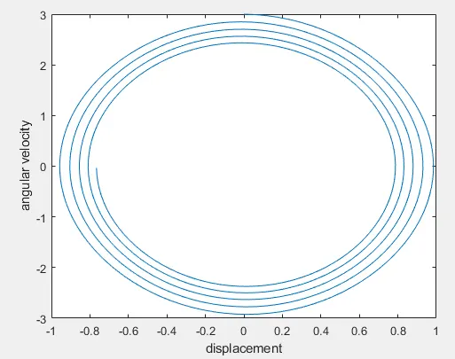
From above figure we can see that, movement of pendulum. From above figure we analyse that, when displacement is zero, angular velocity is maximum and when angular velocity is zeo then displacement is very less. X-axis be the displacement while Y-axis be the angular velocity.
2. Plot Vs Time & Angular velocity :-
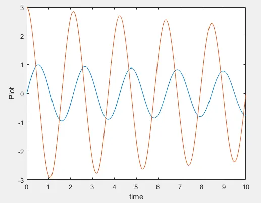
It's the sinosidual wave. Blue wave showing time and red wave showing angular velocity. As time increases, angular velocity decreases and vice-versa. Time starts from zero second while angular velocity starts from 3 rad/sec. It showing the actual movement of pendulum.
3. Pendulum Animation File :-
ERROR DETECTED WHILE CODING :-
1.

This error occurs because video file is not opening, but it directly closed.
2.

This error occurs because of I used ode45 command but not using '@' symbol.
3.
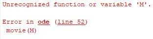
This error occurs due to absence of getframe command in movie file.
4.

This error occurs because of, I mention more variables in main program but less variables in function file.
5.

This error occurs because of combining error of theta1 & theta2 in function file.
SOLUTION ON DETECTING ERROR :-
- In first error, I open the videofile command before closing for the purpose of editing i.e. writting.
- In second error, I mention '@' symbol with ode45, because ode45 is not work seperately.
- In third error, I did not mention getframe command for joining the frame softly. Without it move the pendulum but not close proparly without combining softly.
- In fourth error, I mention equal number of variables in function file and main Matlab code.
- In fifth error, I combining both theta values by using semicolon in function file.
CONCLUSIONS :-
From above code and plot we can analyse following points are-
- ode45 function is used for best precission in values by using fourth and fifth order of Runge-Kutta methods.
- Ode45 function is not run without '@' symbol.
- for best movement of pendulum in second order, ode45 is the best function forever in Matlab.
- getframe command is use to join all the frame softly and close the animation file.
- Input values mentioned in main code and function file must be same.
In this way, I write the code for second order ODE of pendulum, plot the figures as above, created animation file, faced different error and solve that correctly as mentioned above.