Week 3 - Solving second order ODEs

AIM: To Solve a second order PDE for a swinging pendulum with damping effect.

THEORY:

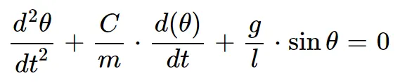
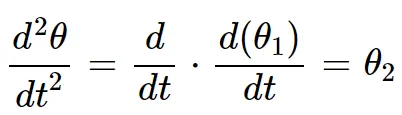
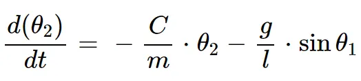
A motion of a pendulum is a second order PDE and cannot be easily solved using python directly. The second order function has to be reduced to two first orders which can be solved by matrix and inbuilt ode function.

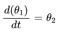
Lets assume;

θ=θ1

The PDE of pendulum is given by;

.......1

........2

The above 1 and 2 equations are the set of two first order equations which has to be solved.

The unknown term here is theta and it is of second order so the initialization is done taking theta as variable:

theta_0 = [0,3]

where 0 is the angular displacement and 3 is the angular velocity in rad/s.

The boundary conditions are as follows:

damper = 0.05
gravitationl_constant = 9.81
length_of_string = 1
mass_of_ball = 1

The program is shown below;

import numpy as np
from scipy.integrate import odeint
import math
import matplotlib.pyplot as plt

#Defining a function for ode
def model(theta,time,damper,gravitationl_constant,length_of_string,mass_of_ball):

	theta1 = theta[0]
	theta2 = theta[1]
	dtheta1 = theta2
	dtheta2 = -(damper/mass_of_ball)*theta2 - (gravitationl_constant/length_of_string)*math.sin(theta1)
	dtheta = [dtheta1,dtheta2]
	return dtheta

damper = 0.05
gravitationl_constant = 9.81
length_of_string = 1
mass_of_ball = 1

#initial_conditions
theta_0 = [0,3]

#points_in_time_range
time = np.linspace(0,20,200)

theta = odeint(model,theta_0,time,args = (damper,gravitationl_constant,length_of_string,mass_of_ball))
plt.plot(time,theta[:,0],'b-',label='Angular Displacement')
plt.plot(time,theta[:,1],'r--',label='Angular Velocity')
plt.ylabel('Plot')
plt.xlabel('Time')
plt.legend(loc='best')
plt.show()

#Animation
x0 = 0
y0 = 0
count = 0
for i in range(len(time)):
	x1 = x0 + length_of_string*math.sin(theta[i,0])
	y1 = y0 - length_of_string*math.cos(theta[i,0])
	filename = str(count) + '.png'
	count = count + 1

	plt.figure()
	plt.plot([x0,x1],[y0,y1])
	plt.plot(x1,y1,marker='o',markersize=10)
	plt.xlim(-1,1)
	plt.ylim(-1.25,0.25)
	plt.savefig(filename)

RESULTS:

The Motion plot over time is shown here:

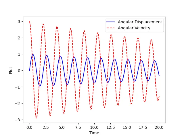
Here we can see that due to damping effect the angular displacement and angular velocity are reducing over time which will settle down after a while.

Video link:https://youtu.be/HAWlnxZyptY

CONCLUSION:

The program was ran in python and second order PDE was solved.