Week 3 - Solving second order ODEs

A Python program to solve the differential equation which governs a simple pendulum

AIM:

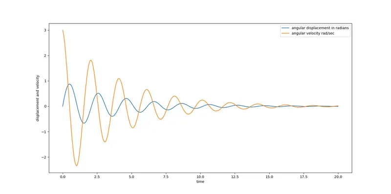
• Simulate the motion between 0-20 sec, for angular displacement=0,angular velocity=3 rad/sec at time t=0.
• Solve the Ode to find out the displacement and velocity of the given initial conditions and time limit.

Briefing:

The governing equation of the simple pendulum is given by :

`(d^2theta)/dt^2 + (b/m)(d theta)/(d t) + g sin theta/L = 0`

Since this is 2nd order ODE, the differential equation needs to be divided into 2 first-order ODE's.

`theta = theta 1`

`(d theta )/ (d t) = (d theta1)/dt = theta2` -------eq 1

`(d^2theta)/ (dt^2) = (d^2theta1)/ (dt^2) = (d theta2)/ dt`

`(d theta2 )/ (dt) + (b/m)theta2 + g(sin theta1) = 0`

The 2 first order ODE's are :

`(d theta1)/dt = theta2`

`(d theta2)/dt = - (b/m) theta2 - g/Lsin theta1`

These two equations are solved separately and the inputted into the odeint function in python, which returns the `theta1 and theta 2`

Steps to program and challenges:

• Import the required modules such as scipy, numpy and also odeint function
• Input the variables such as damping coefficient, gravity, length of the pendulum, and mass of the bob.
• Intialize the boundary conditions which are angular displacement = 0 and velocity = 3.
• Input the time limit which is, in this case, is 20 seconds.
• Using this function : theta = odeint(model, theta_intial,t, args =(b,g,l,m)), the ode is solved by calling the model function.
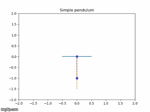
• To simulate the movement of the pendulum, we use a displacement solution vector and loop through each point, then save each plot as separate files

# Program to find the angular displacement and velocity of a simple pendulum from the governing differential equation.

import numpy as np 
from scipy.integrate import odeint
import matplotlib.pyplot as plt 
import math

def model(theta,t,b,g,l,m):
	# seperating the theta intial (90,0) send as one theta into the separete variable
	theta1 = theta[0] 
	theta2 = theta[1]

	#separating the 2nd ode into 2 first order ode's so that 
	dtheta1_dt = theta2
	dtheta2_dt = - (b/m) * theta2 - (g/l)*math.sin(theta1)

	# again puttin thetas together for returning
	dtheta_dt = [dtheta1_dt,dtheta2_dt]

	return dtheta_dt

b = 0.05 # damping coeffient
g = 9.81 
l = 1
m = 0.1 

#intial conidition for both the ode's
 
theta_intial = [0, 3] # (theta1, dtheta1) (disp = 0, velo = 3) pendulum goes from rightside to left

t = np.linspace(0,20,300) 

#solve

# odeint is function in scipy where the args are (funtion which represent the ode,intial coniditon, time limit, other input variables)
theta = odeint(model, theta_intial,t, args =(b,g,l,m))

plt.plot(t,theta[:,0], label = 'angular displacement in radians')
plt.plot(t,theta[:,1],label = 'angular velocity rad/sec')
plt.xlabel('time')
plt.ylabel('displacement and velocity')
plt.legend()
plt.show()
print("angular disp",theta[:,0])

ct = 1

for i in theta[:,0]: # loop through displacement array
	# print('vales of i',i)
	
	filename = str(ct) + '.png'
	ct = ct + 1
	x1=0 # pivot
	y1=0
	x2 = l*math.sin(i) # end point of the pendulum for x axis changes with angular displacement
	y2 = -l*math.cos(i)
	print(x2,y2)
	plt.figure()
	# plt.plot([x1,x2],[y1,y2],color='red')
	plt.plot([x1,x2],[y1,y2],color='blue', marker='o')
	plt.plot([-0.5,0.5],[0,0], label='Simple pendulum with intial velocity 3 rad/sec')
	plt.plot([0,0],[0,-1.5],'--')
	plt.xlim(-2,2)
	plt.ylim(-2,2)
	plt.title('Simple pendulum')
	plt.savefig(filename)

Results:

• The angular displacement and the velocity for the given boundary were found out and plotted.
• The pendulum was simulated using the displacement vector and converting it into the position of the endpoint of the bob.