Week 3 - Solving second order ODEs
AIM:
To solve a second order differential equation using Matlab with the example of a simple pendulum which depicts the motion of it and plot the graph and animation of the same.
THEORY:
Ordinary Differential Equations (ODEs) - It is a differential equation containing one or more functions of one independent variable and the derivatives of those functions. The term ordinary is used in contrast with the term partial differential equation which may be with respect to more than one independent variable.
Simple Pendulum - The simple pendulum is an idealized mathematical model of a pendulum.This is a weight (or bob) on the end of a massless cord suspended from a pivot, without friction. When given an initial push, it will swing back and forth at a constant amplitude. Real pendulums are subject to friction and air drag, so the amplitude of their swings declines.
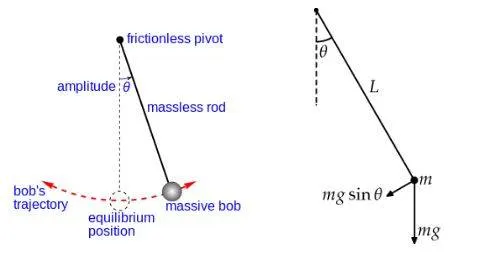
The point from which the bob is suspended is known as point of suspension. Weight of the bob acts vertically downwards and the tension acts vertically upwards, so, the bob comes under equillibrium position and the bob starts oscillating if even smaller external force is applied.
GOVERNING EQUATIONS:
θ is the angle made by the movable link with vertical axis.
L is the length of the movable rod, m is the mass of bob , b is damping coefficient of the system.

To solve this ODE we need to reduce the order of equation into lower order
let θ = θ1
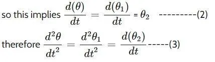
Putting the value of (2) and (3) in (1) , we get-



OBJECTIVES:
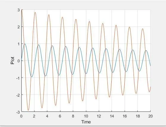
- To solve the second order ODE with graph of Velocity and Displacement in Y axis vs Time in X axis.
- To create the animation of the simple pendulum.
MATLAB CODES:
(i)Code Function for ODE 45 for the main function:
function[dtheta_dt] = ode_func(t,theta,b,g,l,m)

theta1 = theta(1)
theta2 = theta(2)
dtheta1_dt = theta2;
dtheta2_dt = -(b/m)*theta2-(g/l)*sin(theta1);
dtheta_dt = [dtheta1_dt;dtheta2_dt];
end
1. A function is created for ode45 with function name ode_func.
2. theta1 = theta(1)
theta2 = theta(2)
theta(1) is defined as the angular displacement and it is assigned to theta1.
theta(2) is defined as the angular velocity and is assigned to theta2.
3. dtheta1_dt = theta2;
dtheta2_dt = -(b/m)*theta2-(g/l)*sin(theta1);
dtheta_dt = [dtheta1_dt;dtheta2_dt];
Since we have broke the 2nd order equation into two first order equations as shown in the above equations. dtheta =_dt gives the combined column matrix of dtheta1_dt and dtheta2_dt.
(ii)Main Program:
clear all
close all
clc

% Initial inputs:

b = 0.05;
g = 9.81;
l = 1;
m = 1;

% Initial conditions
% Two first order ODE's
% First- Displacement ; Second- Velocity

theta_0 = [0;3];

% Time span
t_span = linspace(0,20,500);

%f= @(t,theta) [theta(2);-(b/m)*theta(2)-(g/l)*sin(theta(1))]

% ODE function definition / calling the function:

[t,results] = ode45(@(t,theta)ode_func(t,theta,b,g,l,m),t_span,theta_0);

figure(1)
hold on;
plot(t,results(:,1))
plot(t,results(:,2))
xlabel('Time');
ylabel('Plot');
grid on;

% To show the displacement results
displ = results(:,1);

% Code for pendulum
ct =1;

for i=1:length(t);

    % Initial position of the pendulum
    x0 = 0;
    y0 = 0;

    %Final position of the pendulum
    x1 = l*sin(displ(i))
    y1 = -l*cos(displ(i))

    % Plotting the 2nd figure:
    figure(2);

    % Base line
    plot([-1 1],[0 0],'linewidth',2,'color','r')

    hold on

    % Pendulum string
    plot([x0 x1],[y0 y1],'linewidth',2,'color','r')

    % Pendulum ball
    plot(x1,y1,'marker','O','markersize',25)

    %Axis fixing in plot
    axis([-2 2 -2 2])
    pause(0.02);
    hold off

    % frame

   M(ct) = getframe(gcf);
   ct = ct+1;
end


movie(M);
videofile = VideoWriter('Pendulum_oscillation.avi')
open(videofile);
writeVideo(videofile,M);
close(videofile);
1. Initial input values are given:
l = 1
m = 1
b = 0.05
g = 9.81
2. theta_0 = [0;3];
The initial values of angular displacement and angular velocity of 0 and 3 have been assigned to theta_0
3. t_span = linspace(0,20,500);
Next is the time span of the total oscillations which is inputted with the linspace function from 0s->20s with calculating 500 intervels in between them.
4. [t,results] = ode45(@(t,theta)ode_func(t,theta,b,g,l,m),t_span,theta_0);
This is the main function given to calculate the total angular displacement and velocity with respect to the given time intervel. The default format of ode45 is [t,y] = ode45(odefun,tspan,y0).
Here, ode is a function of t and theta.
@--> Anonymous functions can accept multiple inputs and return one output. They can contain only a single executable statement.
ode_func(t,theta,b,g,l,m) -->> This is used to call the function ode_func created.
5. figure(1)
hold on;
plot(t,results(:,1))
plot(t,results(:,2))
xlabel('Time');
ylabel('Plot');
grid on;
These are the functions which are used to plot the graph.
figure(1) represents the first figure which has to be plotted.
hold on command helps to plot all the graph in same figure.
plot(t,results(:,1)) # plot of angular displacement and time
plot(t,results(:,2)) # plot of angular velocity and time
6. displ = results(:,1)
All the angular displacement values are stored in a variable named displ
7. for i=1:length(t);
A for loop is created with ct=1 from 1 to last value of t. length(t) defines the total number of values in theta 1. The main advantage is that it is not considered as an array.
8. x0 = 0;
y0 = 0;
x1 = l*sin(displ(i))
y1 = -l*cos(displ(i))
Initial and final values of pendulum has been inputted.
9. figure(2)
Now all the below plots will be done in figure 2
plot([-1 1],[0 0],'linewidth',2,'color','r')
This is the plot for drawing the base line in x axis from -1 to 1.
10 plot([x0 x1],[y0 y1],'linewidth',2,'color','r')
This is the command for plotting the string of the pendulum.
string starts from (x0,y0) and ends at (x1,y1) with a linewidth of 2 and denoted by the colour 'r'.
11. axis([-2 2 -2 2])
pause(0.02);
hold off
The axis is plotted where the graph to be positioned with a pause of 0.02 and the hold is turned off.
12. M(ct) = getframe(gcf);
ct = ct+1;
The first command will create the frame generated into animations.
counter is incremented by one till the iteration stops.
13. movie(M);
videofile = VideoWriter('Pendulum_oscillation.avi')
open(videofile);
writeVideo(videofile,M);
close(videofile);
These are the functions used to create a videofile in avi format.
14. The command window will have 500 values for X and Y between the time period of 20s.
GRAPH PLOTS:
ANIMATION FILE:
ERRORS FORMED:
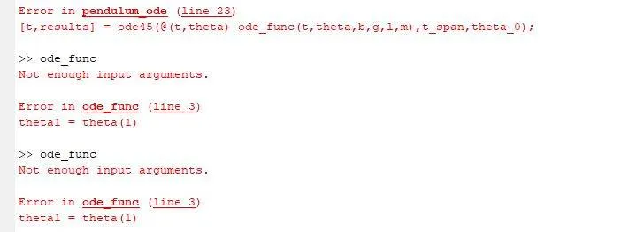

Errors formed due to the case sensitive characters and paranthesis have only been encountered.
CONCLUSION:
The 2nd order ode equation has been solved using the example of simple pendulum and the graphs have been plotted.
The animation of the pendulum is also created.