Week 3 - Solving second order ODEs

Aim :

To solve second order differential equation and create animation of oscillating pendulum.

Objective:

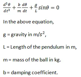
To write a program that solves the following ODE represents the equation of motion of simple pendulum with damping.

Theory:

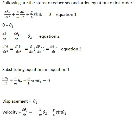
The above equation is second order differential equation. This equation is reduced to a single order equation to solve in MATLAB using the ODE function. ODE is solved based on the Range Kutta method.

The range Kutta method is an effective and widely used method for solving high order differential equations accurately.

clear all
close all
clc

% inputs b=damping , g= gravity, l= length of string, ms= mass of the object,ct is used to save frames. .
b=0.05;
g=9.81;
l=1;
ms=1;
ct=1;

% Initial condition values of displacement and velocity is 0 and 3rad/sec respectively
theta_0 = [0;3];

% To get time points 100 values from 0 to 20 seconds using linspace function
t_span = linspace(0,20,100);

%solve ODE function by geting data from ode_func 
[t, results] = ode45(@(t,theta) ode_func(t, theta,b,g,l,ms), t_span, theta_0);

% plotting graph time against displacement
figure(1)
d=plot (t,results(:,1));
hold on

% plotting graph time against velocity
v=plot(t, results(:,2));
ylabel('plot')
xlabel('time')
legend([d,v],'Displacement','Velocity');

%to animate oscilation of pendulum by fecting value of displacement from ode result
theta = results(:,1);
 for i = 1 : length(theta)
     D = theta(i);

    figure(2)
    %initial values
    x0 = 0;
    y0 = 0;
    % ball end values
    x1 = l*sin(D);
    y1 = -l*cos(D);
   
    plot([x0 x1],[y0 y1],'linewidth',2)
    hold on 
    plot (x1,y1,'o', 'markersize', 10)
    hold off
    axis ([-1.5 1.5 -1.5 1.5])
    pause(0.05)
    m(ct) = getframe(gcf);
    ct = ct+1;
    
 end     
 movie(m)
 videofile = VideoWriter('pendulum_Oscilation.avi', 'uncompressed AVI');
 open(videofile)
 writeVideo(videofile,m)
 close(videofile)

function [dtheta_dt] = ode_func(t,theta,b,g,l,m)

theta1 = theta(1)
theta2 = theta(2)
dtheta1_dt = theta2;
dtheta2_dt = -(b/m)*theta2 - (g/l)*sin(theta1);
dtheta_dt = [dtheta1_dt; dtheta2_dt];
end

Result:

Please find the graph time against displacement and velocity attached in the attachment and animation of the pendulum oscillating video link.

video link:https://drive.google.com/file/d/1XM1vVRJCrdrrm4g_1r5_dSCFLV3sIh6n/view?usp=sharing

Conclusion: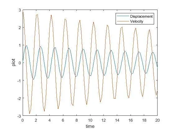

Velocity and displacement vary proportionately with time and create sinusoidal wave wrt time.