Week 3 - Solving second order ODEs

AIM:

To write a program in MATLAB to solve the given ODE and to simulate a motion of the pendulum with the given parameters.

ORDINARY DIFFERENTIAL EQUATIONS (ODE):

An ordinary differential equation is one containing one or more functions of an independent variable and derivatives of that function. Among ODE's, linear differential equations play a vital role. Most of the solutions of physics and maths deal with the solutions from various linear differential equations. Here we are using ODE to solve a function relating to the oscillation of a pendulum with respect to time and angle.

The pendulum oscillation with damping is based on the ODE `(d^2 theta)/dt^2 +b/m (d theta)/dt + g/L sin theta = 0`

Where b - damping co-efficient

g - acceleration due to gravity (m/s^2)

L - Length of the string (m)

m - mass of the bob (Kg)

PENDULUM OSCILLATION:

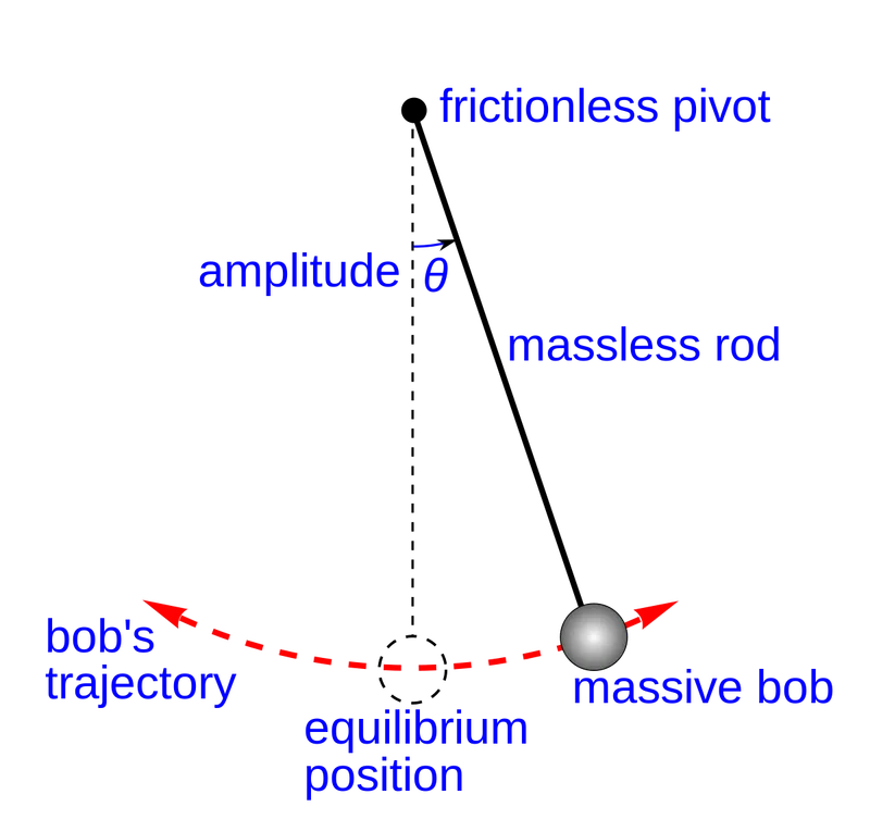
A pendulum is nothing but a ball of some mass 'm' suspended from a point with the help of a string of length 'l'. The pendulum uses the restoration force acting on the ball of mass (Bob) to oscillate about an equilibrium. The time taken for the bob to move over the suspended angle is given by the parameters time and theta. We resolve the ODE to get output parameters like "Angular displacement" and "Angular Velocity" from which we consider angular displacement to express the pendulum's position with respect to the angle theta. The visual of a pendulum is given below.

SOLVING THE ORIGINAL ODE:

Let us assume that `theta = theta_1` and so ,

`(d theta)/dt = (d theta_1)/dt = theta_2` ------> (1)

then, `(d^2 theta)/dt^2 = (d^2 theta_1)/dt^2 = d/dt ((d theta_1)/dt) = d/dt (theta_2)` -------> (2)

Applying this in the original equation and solving we get two ODE solutions, they are

After substitution in original equation -> `(d theta_2)/dt + b/m theta_2 + g/L sin theta_1 = 0`

Solution: 1. `(d theta_1)/dt = theta_2`

2. `(d theta_2)/dt = - b/m theta_2 - g/L sin theta_1`

Therefore, with the solved ODE, we create a function to be solved by the solver ode45. The resulting output gives the value of "Angular displacement" and "Angular Velocity".

We take the values of angular displacement to create the animation because only the displacement matters while plotting the oscillation of the pendulum.

MAIN CODE:

clear all
close all
clc
% Input parameters 
b = 0.05; %Damping co-efficient 
g = 9.81; %Acceleration due to gravity
l = 1;    %Length of the string
m = 0.1;  %Mass of the bob

%Initial displacement and velocity
theta_0 = [0;3];

% Time plot
t_span = linspace(0,20,150);

% ODE solver, using ode45
[t,results] = ode45(@(t,theta)ode_func(t,theta,b,g,l,m),t_span,theta_0);

%Plotting
figure(1)
plot(t,results(:,1)) %Plots the values of entire 1st column
hold on
plot(t,results(:,2)) %Plots the values of entire 2nd column
xlabel('Plot')
ylabel('Time')
legend('Angular Displacement','Angular Velocity')

%Counter initiation
ct = 1;

%Looping
for i = 1:length(t)
    swing = results(:,1);
    SWING = swing(i)
    
    x = 0;
    y = 0;
    
    x1 = l*sin(SWING);
    y1 = -l*cos(SWING);
    
    %Plotting
    figure(2)
    plot([x x1],[y y1],'linewidth',4,'color','b')%String
    hold on
    plot([1 -1],[0 0],'linewidth',4,'color','green')%Top bar
    plot(x1,y1,'O','markers',25,'markerfacecolor','red') %Bob
    axis([-2 2 -2 1])
    pause(0.02)
    hold off
    M(ct)=getframe(gcf)%Getting each frame of oscillation
    ct = ct + 1 %Counter increment
    grid on 
end
%Animation
movie(M)
videofile = VideoWriter('animation_of_pendulum','uncompressed AVI')
open(videofile)
writeVideo(videofile,M)
close(videofile)

FUNCTION USING THE ode SOLVER:

function[dtheta_dt] = ode_func(t,theta,b,g,l,m)
theta1 = theta(1)
theta2 = theta(2)
dtheta1_dt = theta2;
dtheta2_dt = -(b/m)*theta2 - (g/l)*sin(theta1);
dtheta_dt = [dtheta1_dt ; dtheta2_dt]; 
end

CODE EXPLANATION:

1. Initially, we give the values for input parameters like damping co-efficient (b), acceleration due to gravity (g), length of the string (l) and, the mass of the pendulum's bob (m).

2. We define the values of initial displacement and initial velocity

3. We give the time span for the oscillation using "linspace" command setting 500 values to be taken within a span of 0 to 20 seconds.

4. The ode solver, ode45 is given with the function call involving parameters given initial (b,g,l,m, theta, time span). The ode function is called as a separate program which involves the solved ODE's equation as mentioned above as equations (1) and (2). The function calling program can be seen above (ode_func).

5. The output is saved in [t, results] which gives the corresponding solved values of Angular Displacement and Angular Velocity.

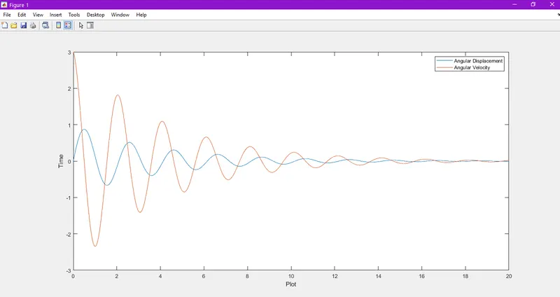
6. They are plotted in a graph in terms of time and the plot. The output is attached below in the results.

7. Since there are 500 values of time to make plots and convert them into an animation, we use a counter. We give the initial value of the counter (ct) as 1.

8. Then since the angular displacement has to be plotted for all 500 values of time, it is given inside a for-loop.

9. The base co-ordinates x and y are given as 0 and x1 and y1 are given with respect to the sin and cos of the respective angle.

10. The animation plot requires the pendulum model and we use plot commands to plot the various components of the pendulum such as the top bar, string, and the bob respectively. The bob is given using 'marker' command and the color is given using 'markerfacecolor'.

11. The axis limits are specified and the commands hold on and hold off help in holding the lines and bob together in the due course of animation and releasing them respectively.

12. We get the individual frame of the 500 plots using getframe(gcf) command and storing it in the movie variable M.

13. Then the animation commands are given as above and is created into an animation file.

ERRORS FACED AND RESOLVING:

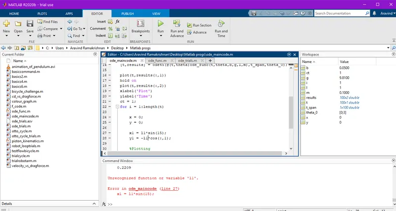
1. Giving l1 instead of length (l) because the co-ordinates are x1 and y1.

2. Placing the hold on after the string plot, which makes it invisible during motion.

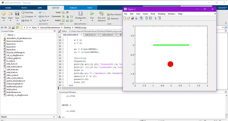
Both errors can be solved by running the code as and when a set of commands is coded, to evaluate correctness then and there instead of running the whole program on a wrong code and replacing it then.

RESULTS:

1. The graph of variations in angular displacement and angular velocity with respect to time is shown below.

2. The animation file running in the plot command.

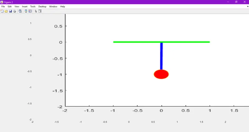
• YOUTUBE LINK TO ANIMATION OF PENDULUM OSCILLATION: https://youtu.be/eAe2cpZ3ALg

CONCLUSION:

Thus we have solved the ODE using the solver ode45 using Matlab. The graph is plotted for the angular displacement and angular velocity along with a plot for the animation of the pendulum's oscillation. Likewise, we can use these solvers to solve any differential equation within seconds. The time taken to solve using Matlab is very quick compared to manual calculation. This can help to solve and simulate any equation within a shorter time thereby creating more time and energy to explore other parameters to be made sure of.