Week 3 - Solving second order ODEs

#Aim:To write a program in MATLAB/Octave that solves the following ODE for a Simple Pendulum.

ODE for simple Pendulum is :

`(d^2(theta))/(dt)^2+(b/m)(d(theta))/(dt)+(g/L)sin(theta)=0` ---------------------------------eq(1)

In the above equation,

g = gravity in m/s2,

L = length of the pendulum in m,

m = mass of the ball in kg,

b=damping coefficient.

#Procedure:

Above equation is second order ODE,we will convert it into first order ODE;

Let's say;

`theta=theta1`

`(d(theta))/(dt)=(d(theta1))/(dt)=theta2` -------------------------------------------------------eq(2)

`(d^2(theta))/(dt)^2=(d^2(theta1))/(dt)^2=d/(dt)(d(theta1))/(dt)=(d(theta2))/(dt)` ----------eq(3)

From eq(2) and (3) ,eq(1) becomes:

`(d^2(theta1))/(dt)^2+(b/m)(d(theta1))/(dt)+(g/L)sin(theta1)=0`

`(d(theta2))/(dt)+(b/m)(theta2)+(g/L)sin(theta1)=0`

`(d(theta1))/(dt)=theta2` -------------------------eq(4)

`(d(theta2))/(dt)=-(b/m)(theta2)-(g/L)sin(theta1)` -------------------------eq(5)

Arrange eq (4) and (5) in Matrix form,for solving;

`d/dt*[[theta1],[theta2]]=[[theta2],[-(b/m)*theta2-(g/L)*sin(theta1)]]`

-------------------------------------------------*************-------------------------------------------------

#Steps followed in code below:

1.All required constants defined as told in challenge and some other variables also defined.

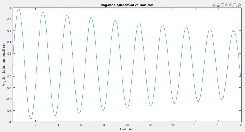
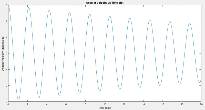
2.Initial condition set: angular displacement=0,angular velocity=3 rad/sec at time t=0.

theta_0[1]= angular displacement

theta_0[2]=angular velocity

3.Function with name 'pendulum_ode_fun' is defined which take (theta,t,b,g,m,l) as input variables and return dtheta1_dt and dtheta2_dt both ODE values as dtheta_dt.

4.Time interval for running simulation set and time interval divided into 200 parts between 0-20.

5.Solver 'ode45' used

'odeint' takes function ,initial condition,time

function=pendulum_ode_fun

initial condition=theta_0

time=t

6.After getting angular displacement and velocity as theta[:,1] and theta[:,2],x and y coordinates of bob(ball) calculated.

7.Then plots for variation of Angular displacement and velocity coded.

9.At last for creating animation of complete simple pendulum motion,code was written and image at every timestep saved for creating animation.

-------------------------------------------**********************------------------------------------------

clear all
close all 
clc

%Main Program Pendulum challenge 

%Constants defined:
b=0.05;					%Damping coefficient
g=9.81;					%Acceleration due to gravity
m=1;					%Mass of ball
l=1;					%Length of string


%Other values used in program for plotting
x0=0;
x1=0.2;
x2=-1.1;
x3=0.08;
x4=-1;
x5=1;

M=[x4,x5,x5,x4,x4];
N=[x0,x0,x3,x3,x0];
%Initial condition
theta_0=[0;3];

%Time intervals
t_span=linspace(0,20,200);

%solve ode
[t theta]=ode45(@(t,theta) pendulum_ode_fun(t,theta,b,g,l,m),t_span,theta_0);

%List defined to store values of bob x and y coordinates from Angular displacement(theta)
bob_x_coordinate=[];
bob_y_coordinate=[];
for j=1:length(t);
	bob_x_coordinate=[bob_x_coordinate (-l*sin(theta(j,1)))];
	bob_y_coordinate=[bob_y_coordinate (-l*cos(theta(j,1)))];
end

%Figure number defined
figure(1)
plot(t,theta(:,1))
xlabel('Time (sec)')
ylabel('Angular displacement(radians)')
title('Angular displacement vs Time plot')
figure(2)
plot(t,theta(:,2))
xlabel('Time (sec)')
ylabel('Angular Velocity(radians/sec)')
title('Angular Velocity vs Time plot')

%Counter variable defined
ct=1;
for i=1:(length(t)-1);
f=figure('visible','off');                          %Figure window will not be displayed
hold on;
plot(M,N);
patch(M,N,'red');
plot([x0,x0],[x1,x2],'color','black','linestyle','--')
plot([x0,bob_x_coordinate(i)],[x0,bob_y_coordinate(i)],'linewidth',2,'color','black');
plot(bob_x_coordinate(i),bob_y_coordinate(i),'marker','o','markersize',20,...
    'markeredgecolor','black','markerfacecolor','blue');
q=quiver(bob_x_coordinate(i),bob_y_coordinate(i),(bob_x_coordinate(i+1)-bob_x_coordinate(i)),...
    (bob_y_coordinate(i+1)-bob_y_coordinate(i)),0,'color','black','Linewidth',3);
axis off;
title(sprintf('Time: % 0.2f sec',t(i,:)));          %Simulation time shown on plot
filename=sprintf('test%05d.png',ct);                %File name given using counter variable
saveas(f,filename);                                 %Figure for every iteration saved 
ct=ct+1;

end

function [dtheta_dt]=pendulum_ode_fun(t,theta,b,g,l,m)
%function return value dtheta_dt

theta1=theta(1);
theta2=theta(2);
dtheta1_dt=theta2;
dtheta2_dt=-(b/m)*theta2-(g/l)*sin(theta1);
dtheta_dt=[dtheta1_dt;dtheta2_dt];

end

---------------------------------------------******************---------------------------------------------

-----------------------------------------------********************-----------------------------------------

#Animation shown below:

https://drive.google.com/file/d/1YAyTNP9aX6rwp02AAmlger9tExmqjyOl/view?usp=sharing

----------------------------------------------***************-------------------------------------------------

#Errors faced:

1.Index exceeds the number of array elements:

While creating arrow using 'quiver',we have to use current and next coordinates for arrow.So for last value of time,there wont be any next value.Therefore it would give 'Index exceeds the number of array elements'.

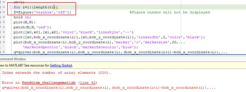
#For rectifying this error,we have to run the for loop shown above for (length(t)-1),not for length(t).

---------------------------------------------**********************--------------------------------