Week 3 - Solving second order ODEs
#Aim:To write a program that solves the following ODE for a Simple Pendulum.
ODE for simple Pendulum is :
`(d^2(theta))/(dt)^2+(b/m)(d(theta))/(dt)+(g/L)sin(theta)=0` ---------------------------------eq(1)
In the above equation,
g = gravity in m/s2,
L = length of the pendulum in m,
m = mass of the ball in kg,
b=damping coefficient.
#Procedure:
Above equation is second order ODE,we will convert it into first order ODE;
Let's say;
`theta=theta1`
`(d(theta))/(dt)=(d(theta1))/(dt)=theta2` -------------------------------------------------------eq(2)
`(d^2(theta))/(dt)^2=(d^2(theta1))/(dt)^2=d/(dt)(d(theta1))/(dt)=(d(theta2))/(dt)` ----------eq(3)
From eq(2) and (3) ,eq(1) becomes:
`(d^2(theta1))/(dt)^2+(b/m)(d(theta1))/(dt)+(g/L)sin(theta1)=0`
`(d(theta2))/(dt)+(b/m)(theta2)+(g/L)sin(theta1)=0`
`(d(theta1))/(dt)=theta2` -------------------------eq(4)
`(d(theta2))/(dt)=-(b/m)(theta2)-(g/L)sin(theta1)` -------------------------eq(5)
Arrange eq (4) and (5) in Matrix form,for solving;
`d/dt*[[theta1],[theta2]]=[[theta2],[-(b/m)*theta2-(g/L)*sin(theta1)]]`
-------------------------------------------------*************-------------------------------------------------
#Steps followed in code below:
1.All required modules are imported.
2.Function name 'model' is defined which take (theta,t,b,g,m,l) as input variables and return dtheta1_dt and dtheta2_dt both ODE values as dtheta_dt.
3.Constants b,g,m,l are defined as told in challenge and some other variables also defined.
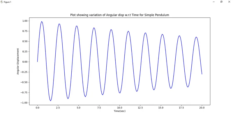
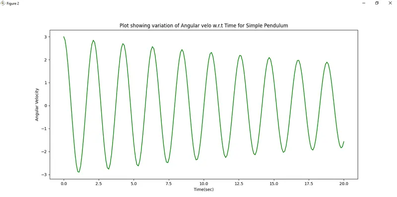
4.Initial condition set: angular displacement=0,angular velocity=3 rad/sec at time t=0.
theta_0[0]= angular displacement
theta_0[1]=angular velocity
5.Time interval for running simulation set and time interval divided into 200 parts between 0-20.
6.Solver 'odeint' called using 'theta'
'odeint' takes function ,initial condition,time
function=model
initial condition=theta_0
time=t
7.After getting angular displacement and velocity as theta[:,0] and theta[:,1],x and y voordinates of bob(ball) calculated.
8.Then plots for variation of Angular displacement and velocity coded.
9.At last for creating animation of complete simple pendulum motion,code was written and image at every timestep saved for creating animation.
-------------------------------------------**********************---------------------------------------
"""
Solve Second order ODE for simple pendulum
(d^2(theta))/(dt)^2+(b/m)(d(theta))/(dt)+(g/L)sin(theta)=0
"""
import numpy as np
from scipy.integrate import odeint
import matplotlib.pyplot as plt
import math


def model(theta,t,b,g,m,l):
	"""
	Function return dtheta1_dt and dtheta2_dt both ODE values as dtheta_dt
	"""

	theta1=theta[0]
	theta2=theta[1]
	dtheta1_dt=theta2
	dtheta2_dt=-(b/m)*theta2-(g/l)*math.sin(theta1)
	dtheta_dt=(dtheta1_dt,dtheta2_dt)
	return dtheta_dt


#Constants defined:
b=0.05					#Damping coefficient
g=9.81					#Acceleration due to gravity
m=1						#Mass of ball
l=1						#Length of string


#Other values used in program for plotting
x0=0
x1=0.2
x2=-1.1
x3=0.08


#Initial condition
theta_0=[0,3]

#Time intervals
t=np.linspace(0,20,200)

#Solve ode
theta=odeint(model,theta_0,t,args=(b,g,m,l))


#List defined to store values of bob x and y coordinates from Angular displacement(theta)
bob_x_coordinate=[]
bob_y_coordinate=[]
for j in range(len(t)):
	bob_x_coordinate.append(-l*math.sin(theta[j,0]))
	bob_y_coordinate.append(-l*math.cos(theta[j,0]))


plt.figure(1)
plt.plot(t,theta[:,0],color='blue')
plt.xlabel('Time(sec)')
plt.ylabel('Angular Displacement')
plt.title('Plot showing variation of Angular disp w.r.t Time for Simple Pendulum')
plt.figure(2)
plt.plot(t,theta[:,1],color='green')
plt.xlabel('Time(sec)')
plt.ylabel('Angular Velocity')
plt.title('Plot showing variation of Angular velo w.r.t Time for Simple Pendulum')
plt.show()

#Counter variable
ct=0

for i in range(len(t)):
	fig = plt.figure(figsize=(15,12))
	ax = fig.add_subplot()
	plt.bar(x0,x3,1,color='w',edgecolor='black',hatch='-+')
	plt.plot([x0,x0],[x1,x2],color='black',linestyle='dashed')
	plt.plot([x0,bob_x_coordinate[i]],[x0,bob_y_coordinate[i]],linewidth=5,color='black')
	plt.plot(bob_x_coordinate[i],bob_y_coordinate[i],marker='o',markersize=20,color='blue')
	ax.annotate("",xy=(bob_x_coordinate[i],bob_y_coordinate[i]), xycoords='data',
	xytext=(bob_x_coordinate[i+1],bob_y_coordinate[i+1]), textcoords='data',arrowprops=dict(arrowstyle="<-",
	connectionstyle="arc3"),)


	ct=ct+1
	filename='test%05d.png'%ct
	plt.title('Time-{0:.3f} sec'.format(t[i]),weight='bold')
	plt.xlim([-2,2])
	plt.ylim([-1.8,0.5])
	plt.savefig(filename)
#Animation shown below:
-------------------------------------------------********************---------------------------------------
#Error faced while programming:
I faced few errors while programming due to:
a.)Docstring-I gave indent where required
b.)Name not defined-Defined variable and corrected spelling at some place.
c.)Invalid syntax error-Colon ,comma's putted where required
##One error was coming continuously,shown below:
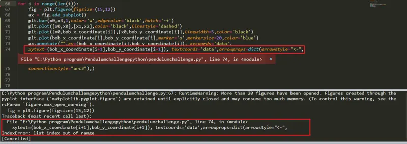
For rectifying error,i ran for loop for 'len(t)-1'.It worked.
--------------------------------------------*****************-------------------------------------------------