Solving second order ODEs

Solving Second Order Ode's

Aim:

To able to write the python program to simulate the pendulam motion by using second order ordinary differential equation and create the animation of simple pendulam by using the imagic magic software.

Softwares required:

1.Python

2.Sublime text editor

3.ImagicMagick

Theory:

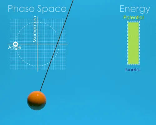
The Simple Pendulam:

A simple pendulum is defined, ideally, as a particle suspended by a weightless string. Practically it consists of a small body, usually a sphere, suspended by a string whose mass is negligible in comparison with that of the sphere and whose length is very much grater than the radius of the sphere. Under these conditions, the mass of the system may be considered as concentrated at a point -namely, the center of the sphere- and the problem may be handled by considering the transitional motion of the suspended body, commonly called “bob,” along a circular arc.

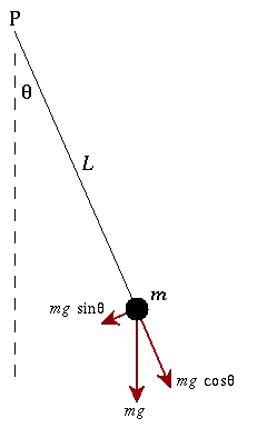A simple pendulum consists of a mass m hanging from a string of length L and fixed at a pivot point P. When displaced to an initial angle and released, the pendulum will swing back and forth with periodic motion. By applying Newton's secont law for rotational systems, the equation of motion for the pendulum may be obtained,and rearranged as. If the amplitude of angular displacement is small enough that the small angle approximation () holds true, then the equation of motion reduces to the equation of simple harmonic motion . The simple harmonic solution is with being the natural frequency of the motion.

Small Angle Approximation and Simple Harmonic Motion:

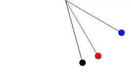With the assumption of small angles, the frequency and period of the pendulum are independent of the initial angular displacement amplitude. All simple pendulums should have the same period regardless of their initial angle (and regardless of their masses). This simple approximation is illustrated in the (48 kB) mpeg movie at left. All three pendulums cycle through one complete oscillation in the same amount of time.

The period for a simple pendulum does not depend on the mass or the initial anglular displacement, but depends only on the length L of the string and the value of the gravitational field strength g, according toThe mpeg movie at left (39.5 kB) shows two pendula, with different lengths. How many complete oscillations does the shorter (blue) pendulum make in the time for one complete oscillation of the longer (black) pendulum? From this information and the definition of the period for a simple pendulum, what is the ratio of lengths for the two pendula?

The Real (Nonlinera) Pendulum:

When the angular displacement amplitude of the pendulum is large enough that the small angle approximation no longer holds, then the equation of motion must remain in its nonlinear form

.

This differential equation does not have a closed form solution, and must be solved numerically using a computer. Mathematica numerically solves this differential equation very easily with the built in function NDSolve[ ].

Small initial Amplitude:

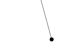The small angle approximation is valid for initial angular displacements of about 20° or less. The (0.132MB) mpeg movie at left shows two pendula: the black pendulum assumes the linear small angle approximation of simple harmonic motion, the grey pendulum (hidded behind the black one) shows the numerical solution of the actual nonlinear differential equation of motion. For small initial angular displacements the error in the small angle approximation becomes evident only after several oscillations.

Large Initial Amplitude:

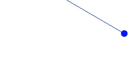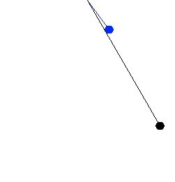
When the initial angular displacement is significantly large that the small angle approximation is no longer valid, the error between the simple harmonic solution and the actual solution becomes apparent almost immediately, and grows as time progresses. In the (0.226MB) mpeg move at left, the dark blue pendulum is the simple approximation, and the light blue pendulum (initially hidden behind the dark blue one) shows the numerical solution of the nonlinear differential equation of motion.

Coordinates of simple pendulam when at initial condition:

>>Fixed point of the simple pendulam (x1,y1) = (0,0)

>>Hanging point of the ball at initial condition (x2, y1) = (L*sin(theta), -L*cos(theta))

Program calculations and its Explinations:

Inputs:

Center of gravity (g) =9.81 m/sec²

^{Length of the pendulam (L) = 1m}

^{Mass of the ball (m) = 1kg}

^{Damping coefficint (b)= 0.05}

^{Motion time = 0-20sec}

^{Angular displacement =0}

^{Angualr velocity = 3 rad/sec}

^{time (t)=0}

Important paramaters and formulaes:

theta1=theta[0]
theta2=theta[1]
dtheta1_dt=theta2
dtheta2_dt=-(b/m)*theta2-(g/2)*math.sin(theta1)

^{Programme for showing the simple pendulam oscillations:}

Initially we need to comment what the programme is about and giving the necessay inputs for defining the functions then convert the second order equation into first order ode. After that all the values are uploded for generating the programme and by using for loop and plotting modules pendulam oscillations are to be created.

import numpy as np
from scipy.integrate import odeint
import matplotlib.pyplot as plt
import math

#function that returns dx/dt
def model(theta,t,b,g,l,m):
	theta1=theta[0]
	theta2=theta[1]
	dtheta1_dt=theta2
	dtheta2_dt=-(b/m)*theta2-(g/2)*math.sin(theta1)
	dtheta_dt=[dtheta1_dt,dtheta2_dt]
	return dtheta_dt

b=0.05
g=9.81
l=1
m=0.1

#initial condition 
theta_0=[0,5]

#time points
t=np.linspace(0,10,150)

#solve
theta=odeint(model,theta_0,t,args=(b,g,l,m))

#plot results
plt.plot(t,theta[:,0],'b-',label=r'$frac{dtheta_1}{dt}=theta2$')
plt.plot(t,theta[:,1],'r--',label=r'$frac{dtheta2}{dt}=-frac{b}{m}theta_2-frac{g}{L}sintheta_1$')
plt.ylabel('plot')
plt.xlabel('time')
plt.legend(loc='best')
plt.show()


y=theta[:,0]

ct=1

for ang in y :
	x1=0;y1=0
	x2=l*math.sin(ang)
	y2=-l*math.cos(ang)
	file='test%05d.png'%ct 
	plt.figure()
	plt.plot([-1.5,1.5],[0,0],linewidth=8)
	plt.plot([x1,x2],[y1,y2],linewidth=3)
	plt.plot(x2,y2,'o',markersize=15)
	plt.xlim([-1.5,1.5])
	plt.ylim([-1.5,1.5])
	plt.savefig(file)
	ct=ct+1

Output:

Angalur velocity and Angular displacement graph with respect to time:

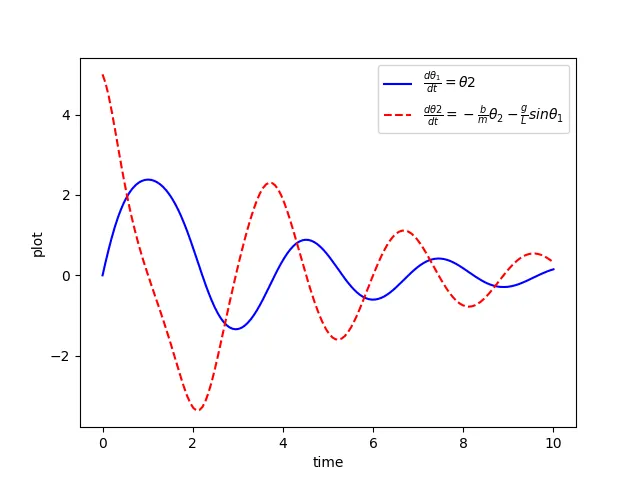
The above graph shows the damping coefficint of the angualr velocity and angular displacement of simple pendulam is decreasing with respect to time.

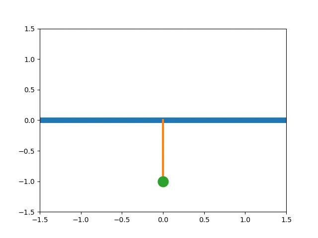
Animation of Simple pendulam oscillations:

Result:

The simulation of pendulam motion by using second order ordinary differential equation and its pendulam oscillations are created sucessfully by using the python sublime text editor imagic magic softwares.