Week 3 - Solving second order ODEs

Pendulum  Animation using 2^nd Order Ode.

Avinash.A ( [email protected])

 

AIM:  

To obtain a virtual motion video of a simple pendulum by solving a second order differential equation with the help of MATLAB.

THEORY:

A simple pendulum is an ideal example of a second order differential equation.

The pendulum keeps swinging with respect to its mean point and eventually gets damped with the help of gravity if its suspended freely at air,

Another similar example for the same is a spring mass system.

The mass keeps oscillating in vertical direction, until it gets damped by the virtue of its spring coefficient or the medium in which its suspended.

The second order function is solved with an inbuilt operator in MATLAB called as ode45.

Methodology :

 

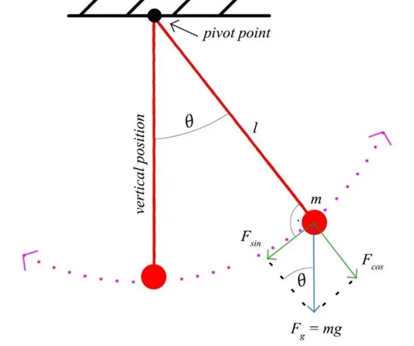
Similar to the above figure 1,

• We consider “l” as the length of the pendulum
• “M” as the mass of the sphere attached
• “theta” as the angle suspended by the pendulum at each positions
•  " g " is acceleration due to gravity.  

the diffrential equation is given as :

`d^2theta/dt + (b/m)d theta/dt + g/l(sin theta)=0`

and then consider `theta=theta1`

hence `d theta1/dt = theta2`

substituting the above value to cnvert the equation to single order we get

hence ,

`d theta2/dt= (-b/m)theta2 - (g/l)sintheta`

MATLAB CODE 1:

function [dtheta_dt] = ode_func(t,theta,b,g,l,m) % defining dunction

theta1= theta(1)
theta2 = theta(2)
dtheta1_dt = theta2;
dtheta2_dt =  -(b/m)*theta2 - (g/l)*sin(theta1);
dtheta_dt = [dtheta1_dt; dtheta2_dt];
end
 

The function is created to the values of the of the diffrential equation by taking the inputs as t (time), theta (angle), b(damping coeff), g ,l(length), and m(mass). this acts as a template for the ode function to act.

MATLAB CODE2:

clear all
close all
clc
%defining inetial conditions
b = 0.05;
g = 9.81;
l = 1;
m = 1;
theta_0 = [0;3];
% the bandwidth of the swing
t_span = linspace(0,20,100);
% solving the ode with the ode45 inbuilt function
[t,results] = ode45(@(t,theta) ode_func(t,theta,b,g,l,m),t_span, theta_0);
figure(1)
% ploting the firt colum and retaining its plot
plot(t,results(:,1))
hold on
grid on
% ploting the second colum and retaining its plot
plot(t,results(:,2))
% giving the perfect fit for the graph
axis([0 20 -3 3])
ylabel('plot')
xlabel('time')
% setting the fixed point of hinge
x0=1;
y0=1;
ct=1;
coord = results(:,1);
for i=1:length(coord)
    figure(2)  % new window 
    % resolving the line in order to get various points of swing
    x1 = 1-l*sin((coord(i)));
    y1 = 1-l*cos((coord(i)));
    % creating a reference line for the hinge
    plot([0,2],[1,1],'linewidth',5)
    hold on
    % line connectng the fixed point to moving point
    plot([1,x1],[1,y1],[x1,x1],[y1,y1],'o','markerfacecolor','r','linewidth',2)
    hold off
    axis([0 2 -0.5 1.5])
    grid on
    pause (0.01)
    % collecting all the frames
    M(ct) = getframe(gcf);
    ct = ct+1;
end
movie(M) % creating the movie file and saving it with a name 2ndode in avi format
videofile = VideoWriter('2ndode.avi','uncompressed AVI');
open(videofile) % open videofile
writeVideo(videofile,M)
close(videofile) %close the videofile

CODE OVERVIEW:

1. clear all the stored values by base commands
2. define the values of damping and lenght of the pendullam with other basic values
3. set the timespam for the program to run.
4. use the inputs of t and theta obtained and use the ode solver function in the matlab, with the function created prior to program and store the result in the array [t,result]
5. plot both the graphs individually by using hold on command.
6. the animation is created by assigning a line with coordinates for the obtained values using the concept of resolution of vectors.
7. also give a fixed point at the hinge and also denote a spehere with radious x repercenting bob.
8. pause command used for looping values.
9. the movie is created and stored in avi format by capturing all the frames.

GRAPH OBTAINED:

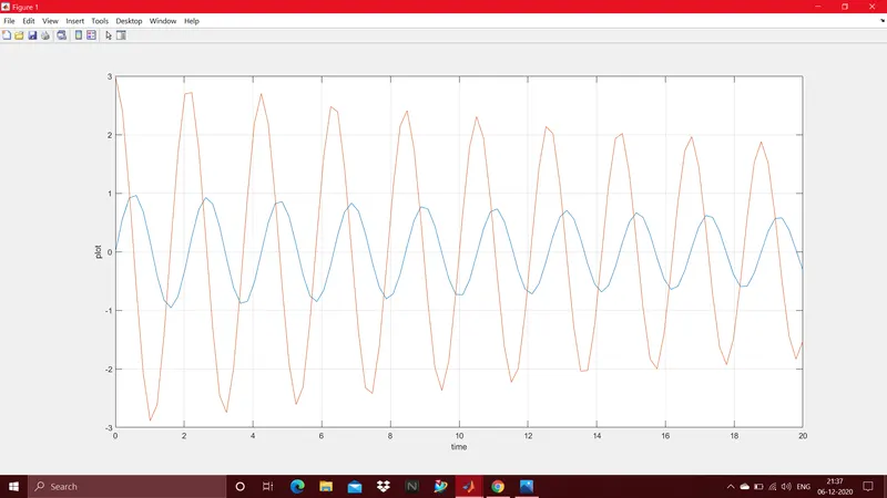
THE RED COLOR REPERCENTS VELOCITY AND THE BLUE COLOR REPERCENTS DISPLACEMENT.

As time pass we see that the graph gets damped due to the damping coefficient and gravity.

videofile:

https://drive.google.com/file/d/18M5k95i95R2JJXi8rVB5pmIB7zjxV1AP/view?usp=sharing

CONCLUSION:

The second order equation given is converted to a motion of pendullam succesfully with the help of matlab and the plot of velocity and displacement variation with time is obtained as attached above.