Week 3 - Solving second order ODEs

Aim: To solve the second order ODE and create an animation of the pendulum based on the results.

Theory: In Engineering, ODE is used to describe the transient behavior of a system. A simple example is a pendulum. The way the pendulum moves depends on the Newtons second law. When this law is written down, we get a second order Ordinary Differential Equation that describes the position of the "ball" w.r.t time.

This ODE represents the equation of motion of a simple pendulum with damping :

(d^2`theta`/dt^2) + (b/m)*(d`theta`/dt) + (g/L)sin`theta`= 0

where b= Damping coefficient,

g = gravity in m/s2,

L = length of the pendulum in m,

m = mass of the ball in kg.

For solving this ODE of the second degree we are first going to write this equation in terms 1st degree ODE's and then use the resulting equations in a function to solve the above equation with the help of the ODE solver 'ode45' in MATLAB . After getting the results , they are used to plot to plot the pendulum by calculating the positions with respect to '`theta`' that is the angular displacement with respect to 't'. Now:

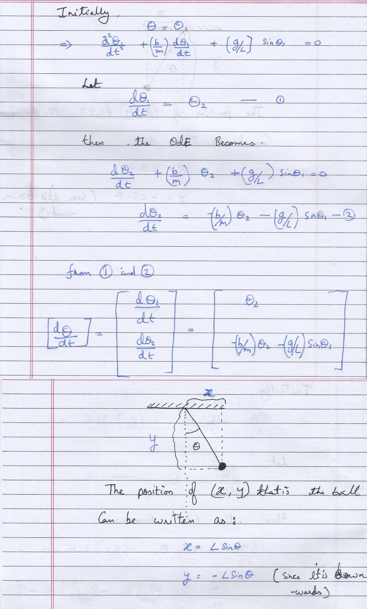
Using the above equations we can now proceed towards writing the required code.

Code:

% Program to solve the 2nd order ODE
clear all 
close all 
clc

% Inputs
%Damping cofficient
b = 0.05;

%Gravity
g = 9.81;

%Length of the arm
l = 1;

%Mass of the ball
m = 0.1;

% Intial condition
theta_0 = [0;3];

% Time points
t_span = linspace(0,20,300);

% Solving ODE using ode45 function and the ode_function which has the 2nd
% degree ODE brokendown into the required equations for the solution
[t , results] = ode45(@(t, theta) ode_function(t,theta,b,g,l,m), t_span, theta_0);
theta = results(:,1);
v_a = results(:,2);
ct = 1;

%Plotting
axis([-2 2 -2 2]);
h = -1;

%The loop to create small Rectangles giving a brick like effect
for i = 1:20
  
   
   rectangle('Position',[h,0,0.1,0.0125],'EdgeColor',[0.5 0.5 0.5]);
   v = 0;
   for j = 1:10
     rectangle('Position',[h,v,0.1,0.0125],'EdgeColor',[0.5 0.5 0.5]);
     v = v + 0.0125;
   end
   h = h + 0.1;
end

%The loop to create the animation of the pendulum
for i = 1:length(t)
    
    x = l*sin(theta(i));
    y = -l*cos(theta(i));
    x0 = 0;
    y0 = 0;
    wall = rectangle('Position',[-1,0,2,0.125],'EdgeColor',[0 .5 .5],'LineWidth',2);
    hold on
    arm = plot([x0 x],[y0 y],'color','r','Linewidth',4);
    ball = plot(x,y,'Marker','o','MarkerSize',15,'MarkerFaceColor','g','MarkerEdgeColor','g'); 
    txt1 = {'Angular displacement=', num2str(theta(i))};
    txt2 = {'Angular velocity=',num2str(v_a(i))};
    displacement = text(0.5,1,txt1);
    vel = text(-1.5,1,txt2);
    
    M(ct) = getframe(gcf);
    ct = ct+1;
    
    %For deleting overlap in the animation at different positions
    delete(arm);
    delete(ball);
    delete(displacement);
    delete(vel);
    
end

% Creating the video file
movie(M);
videofile = VideoWriter('Pendulum.avi','Uncompressed AVI');
open(videofile);
writeVideo(videofile , M);
close(videofile);

Code function:

function [dtheta_dt] = ode_function(t,theta,b,g,l,m)
    
    theta1 = theta(1);
    theta2 = theta(2);
    dtheta1_dt = theta2;
    dtheta2_dt = -(b/m)*theta2-(g/l)*sin(theta1);
    dtheta_dt = [dtheta1_dt ; dtheta2_dt];

end

Code Explanation: I have started the code with 'clear all', 'close all', 'clc' these three a very helpfull as there might be many open windows or outputs when trying out the code in initial stages also automatically closes, clears any and all already open windows or outputs before running the rest of the code .

Then for the next step i have taken the given inputs and assigned them to the respective variables.

Here the variable 'theta_0' represents the initial dispalcement and the initial angular velocity and is stored as a column matrix and this is important as it is an integral part in the program to remember as it is the input for our function 'ode_function' .

Next the variable 't_span' is an array containing the time 0-20 sec and is created using linspace command.

ode45 : This is a predefined function in MATLAB ,this is a ODE's solver . The syntax for ode45 is:

[t results]= ode45( @(t, theta) ode_function(t,theta,b,g,l,m) ,t_span, theta_0)

`ubrace ` ` ubrace ` ` ubrace`

( This part means that our ODE is a function of t, theta) (The user defined function which provides the relationship) (The input of the integration window and intial conditions )

ode_function: Here we have written down the 2nd order ODE in terms of 2 first order ODE's to solve it . The function is written in terms of the equations 1 and 2 as given in theory.

Now after I get the results it is a matrix with 300 rows and 2 columns, first column being the angular displacement which I then stored in variable named 'theta' and the second column being angular velocity stored in 'v_a'. After this I started the plotting but first i declared a variable 'ct' that is a counter variable.

In the Plotting section i have first set the axes using the axis command . Then I have next written a small loop to create the brick like effect in the wall from which the pendulum is hanging and for this I have used the rectangle command , syntax for the command is 'rectangle('Position',[x y w h],Linespecs......)' where the x and y represent the coordinates where the rectangle starts or positioned and 'w and h' are its width and height with respect to the position. i have written this loop in such a way that for each time the outer loop runs the inner loop runs 10 times stacking up the bricks on each other. den for the next run of the outer loop the position is changed .

After this comes the loop to create the pendulum animation here the loop counter is set such that the loop run for the length of the variable 't' that is time. Then the x and y coordinates of the ball is determined with the help of the the statements 'x = l*sin(theta(i)) and y= -l*cos(theta(i))' and 'x0 and y0' represent the fixed point on the wall . After that i have plotted the wall using rectangle command and stored it in variable 'wall' next i have plotted the arm using plot command and stored it in variable 'arm' similarly i plotted the ball and stored it in variable 'ball'. Next i have created variables 'txt1' and 'txt2' having string values that is the messages 'Angular displacement= and Angular velocity=' and using num2str command i have converted the respective values to string. Using the text command i have dispalyed the dispalcement and velocity and stored them respectively in variables 'displacement' and 'vel'.

The next two lines are to store the current frames or figures here using the counter variable 'ct' i have stored the the current frame in 'M' with the help of the 'getframe' command, then i have incremented the counter variable 'ct'.

Now to so as to get all the above plots in one figure i had to use 'hold on' command but because of the hold on command i had a over lap of the elements so in order to deal with thid i used 'delete' command to delete all overlapping elements those are the 'arm', 'ball' ,'vel' and 'displacement' with these comands the loop ends

Now for the movie i used the movie(M) command, next created a variable 'videofile' and using the command VideoWriter i have made the file named Pendulum.avi file and uncompressed in the nature. Now using the 'open' command i opened the videofile and with the help of writeVideo command i have written 'videofile' with 'M' and then closed the videofile with the help of 'close' command .

Output:

The Pendulum Animation