TO SIMULATE THE BEHAVIOUR OF SIMPLE PENDULUM BY USING PYTHON

AIM

To simulate the transient behaviour of simple pendulum, plotting the angular velocity and displacement with function of time by using PYTHON.

INTRODUCTION

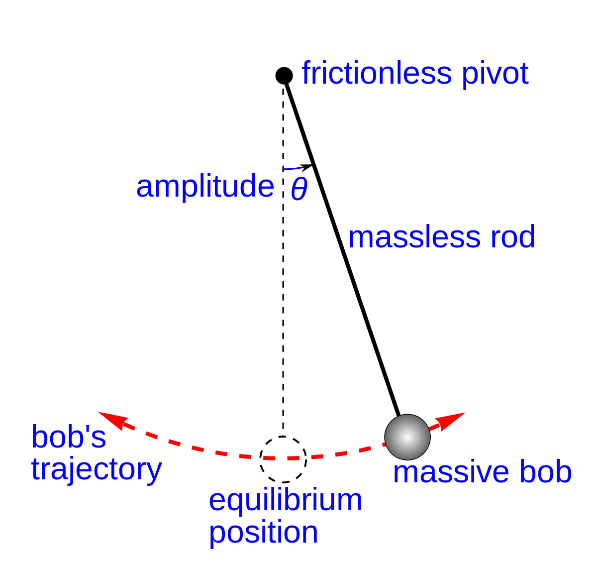
A pendulum is a weight suspended from a pivot so that it can swing freely. When the pendulum is displayed in sideways from its resting, equilibrium position, it is subject to a restoring force due to gravity that will accelerate back toward the equilibrium position. When released, the restoring force acting on pendulum's mass cause it to oscillate about the equilibrium position, swinging back and forth. The time for one complete cycle, a left swing and a right swing is called the period. The period depends on the length of the pendulum and also to a slight degree on the amplitude, the width of the pendulum's swing.

SIMPLE PENDULUM DIAGRAM

DAMPING OSCILLATIONS WITH RESPECT TO TIME

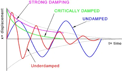
Critically damped - A system moves as quickly as possible toward equilibrium without oscillating about the equlibrium

Undamped - A system oscillates at constant frequency without experiencing decay of its amplitude.

Underdamped - A system moves quickly to equlibrium, but will oscillate about the equilibrium point as it does so.

OBJECTIVE

1) Breakdown into first order differential equation from second order differential equation.

2) Creating a plot of simple pendulum oscillation with respect to time by using angular displacement & velocity.

ODE EQUATION

1) The abbreviation of ode is ordinary differential equation is a differential equation containing one or more functions of one independent variable and the derivates of those functions.

2) For transient motion at any system, the second differential equation is help us to finding the unknown variables at instantenous point in the system trajectory.

3) For finding pendulum motion, this second order differencial equation used and it's written below.

`(d^2theta)/(dt^2)+b/m (d theta)/(dt)+g/l sintheta = 0` ------- 1

Pendulum physical specification

Length, l = 1 m

Mass, m = 1 kg

Damping coefficient, b = 0.05 Ns/m

Acceleration force , g = 9.81 m/sec^2

4) In order to finding the values, convert the equation from second order to first order in mathematically.

`theta = theta1`

`(d theta)/dt = (d theta1)/dt = theta2` ----- 2

`(d^2 theta)/dt^2 = (d^2 theta1)/dt^2 = d/dt((d theta1)/dt) = d/dt(theta2)` ----- 3

Subsitute the 2 & 3 value in equation 1

`(d^2 theta)/dt^2+b/m (d theta)/dt + g/l sintheta = 0`

`(d^2 theta1)/dt^2 + b/m (d theta1)/dt + g/l sintheta1 = 0`

`(d theta2)/dt +b/m theta2 + g/l sintheta1 =0`

`(d theta1)/dt = theta2`

`(d theta2)/dt = -b/m theta2 - g/lsintheta1`

`d/dt[ theta1; theta2] = [theta2;-b/m theta2 - g/lsintheta1]`

PYTHON CODE :

import numpy as np
from scipy.integrate import odeint
import matplotlib.pyplot as plt
import math

# Functions that return dx/dt
def model (theta,t,b,g,l,m):
	theta1 = theta[0]
	theta2 = theta[1]
	dtheta1_dt = theta2
	dtheta2_dt = -(b/m)*theta2 - (g/l)*math.sin(theta1)
	dtheta_dt = [dtheta1_dt,dtheta2_dt]
	return dtheta_dt

b = 0.05
g = 9.81
l = 1
m = 1

# Initial condition
theta_0 = [0,3]

# Time points
t = np.linspace(0,20,200)

# Solve ODE
theta = odeint(model,theta_0,t,args = (b,g,l,m))

# Plot results

plt.plot(t,theta[:,0],'-',label='Angular displacement with respect to time')
plt.plot(t,theta[:,1],'--',label = 'Angular velocity with respect to time')
plt.ylabel('Angular displacement & Angular Velocity')
plt.xlabel('Time in seconds')
plt.title('Transient behaviour of Simple pendulum')
plt.legend()
plt.savefig('Simple pendulum')
plt.show()

ct = 1
for theta in theta[:,0]:
	x0 = 0
	y0 = 0
	x1 = l*math.sin(theta)
	y1 =-l*math.cos(theta)

	Simple_pendulum = 'image %05d.png' % ct
	plt.figure()
	plt.plot([-1,1],[0,0],'black',linewidth = 7)
	plt.plot([x0,x1],[y0,y1],'red',linewidth = 3)
	plt.plot(x1,y1,'o',markersize = 20)
	plt.xlim([-2,2])
	plt.ylim([-2,2])
	
	ct = ct + 1
	plt.savefig(Simple_pendulum)
	#plt.show()

EXPLANATION :

1) Importing the all needed modules like math, matplotlib, numpy and odeint from scipy.integrate.

2) Math module is help to calculate the trigononetric ratios for an angle angle in both radians as well as degree. Matplotlib module is one of the python library with help us to plotting. A numpy module is another one in python library is used for working with arrays.

3) Odeint module import from scipy open source python library, scipy has contains various modules. Odeint, basically a function that will integrate ordinary differential equation or system of ordinary differential equations.

4) Defining a function with 'model' function of damping(b), mass(m), length(l), gravity(g). Under the function we have put derivative, breakdown from second order differential to first order differential equation.

5) Providing the inputs parameters such as damping, mass of the bob, gravity acting on a bob and length of the string.

6) Providing an initial condition which are angular displacement and angular velocity of the bob. Provide the time span from 0 to 20 seconds.

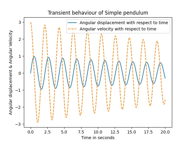
7) Create a 'odeint' function of calling 'model' function, initial conditions, time span and arguments. After completion of calculation, we have two column of outputs till 200 rows. A first column of results is angular displacement with respect to time, a second column is angular velocity with respect to time.

8) By using the results, we has to plotting the oscillation of simple pendulum with respect to time.

9) Create a 'for loop' for which storing the position of simple pendulum in image format. After the each iteration, a counter will execute to next integer.

10) Each iteration, a figure will save with proper labels, legends and limits on both sides.

11) By using image magick software, we should convert from images into gif format.

RESULT AND DISCUSSION :

1) Initial displacement is zero, so that starts from zero corresponds to zero second. Over the period of time, a oscillation was shrinkage due to damping ratio on that simple pendulum.

2) Initial velocity is three, so that starts from three corresponds to zero second. Over the period of time, in velocity also was shrinkage due to decreasing the angular displacement on that simple pendulum.

3) Angular velocity is proportional to angular displacement.

Youtube Video Link : https://youtu.be/0Urc74lyLfs

ERROR FACED WHILE PROGRAMMING :

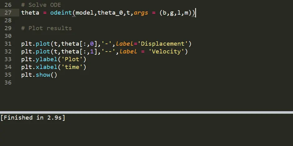
I was forgot to put the end parenthesis at the line number of 27. So that error had pop up like 'invalid syntax' from command window.

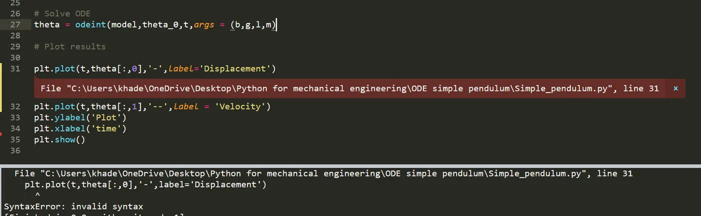
After I put the end parenthesis , couldn't error was popup.

CONCLUSION :

Finally, successfully ran the python code to got the simple pendulum smooth animation. And also got the transient behaviour of simple pendulum with function of angular displacement & velocity and respect to time seconds.