Week 3 - Solving second order ODEs

OBJECTIVE :- To solve second order ordinary differential equations (ODE’s) by using simple pendulum example.

PROBLEM STATEMENT :-

In engineering, ODE is used to describe the transient behaviour of a system. A simple example is a pendulum.

The way the pendulum moves depends on the Newton’s second low When this low is written down, we get a second order ODE that describes the position of the “ball” w.r.t. time.

Similarly, there are hundreds of ODE’s that describe key phenomenon and if we have the ability to solve these equations then we will be able to simulate any of these systems.

Our objective is to write a program that solves the following ODE. This ODE represents the equation of motion of a simple pendulum with damping-

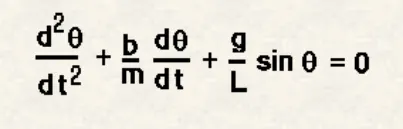
In the above equation-

g = gravity in m/s^2 = 9.81

l = length of the pendulum in m = 1

m = mass of the ball in kg = 1

b = damping coefficient = 0.05

Write a program in python that will simulate the pendulum motion, just like the one shown in the start of this challenge.

Simulate the motion between 0-20 sec, for angular displacement = 0, angular velocity = 3 rad/sec at time t = 0.

When we do this we should get the position of the pendulum as a function of time. Use this information to animate the motion of the pendulum.

1. For each value of the time-

• Create an image that represents the position of the pendulum
• Assume the length of the string and size of the ball.
• Use the marker command to create a sphere
• One end of the pendulum is fixed.
• The other end moves according to the simulation of ODE which we neet to solve.

2. Submit a report that has the following contents-

• Stepwise explaination of code
• Error faced while programming
• How have we overcome those errors
• Screenshots showing errors thrown in command window.

SOLUTION PROCEDURES :-

For writing python code I use following methods-

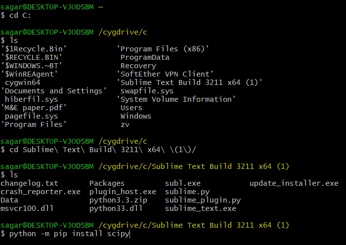
1. To run the program we need scipy command, so that it install by using “python -m pip install scipy” command in python by using cygwin or command promptin python directory.
2. Install matplotlib because we need plotting here.
3. Import odeintto rotate the pendulum bob by angular displacement.
4. Define all the constant and initial conditions in angle I.e theta_0.
5. Define initial conditions to solve second order ODE.
6. For solving both ODE we need to values which is mention in theta_0.
7. First value is for angular displacement and second is for angular velocity.
8. Then define time array by using numpy command.
9. Use the linspace from 0 to 200 I need total 200 images.
10. Then solve the differential equation by using odeint It’s the command inside the scipy module, and if we try to run this command without scipy module then it will not going to work.
11. Odeint is a function which integrate the ODE equation or system of ordinary differential equations.
12. For integrating the ODE we need to define system I.e. our model which we defined already.
13. Then we need to define initial conditions, time arrays and arguments.
14. Model is a function which define ODE as a system.
15. Two differential equations I defined as adtheta1_dt and dtheta2_dt.
16. And then I combine these two equation in dtheta_dt.
17. And then return these dtheta_dt.
18. Theta is our final solution and then plot the results.
19. Here theta1 is a angular displacement and theta2 is a angular velocity.

RESULTS :-

A. Error section :-

While writing python code I get some error as follows-

1. Contour error :- This error occur due to undefined of initial value of contour.

2. Initial condition of theta_0 :- If this conditions not applied proparly then also we get error, because theta_0 value defined angular displacement and angular velocity.

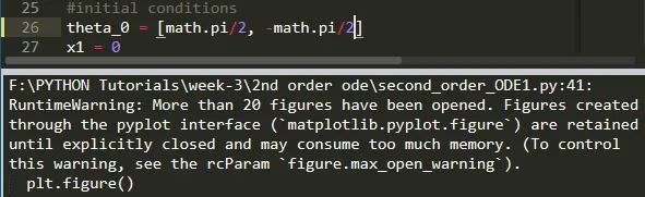
3. Fixed point error :- Pendulum string has two points, if we not defined initial points then also we get error.
4. Defined time array proparly with the help of numpy module and linspace command.
5. Defined theta in odeint, model and arguments.
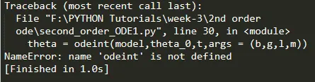
6. If we run odeint command without installing and importing scipy module then also we get error as follows-

7. Theta error :- Also use proper for loop by defining theta because if we not defined angular displacement and angular velocity then we get error as follows-

8. For plotting fixed the X and Y axis range.
9. Use marker command to create a sphere.

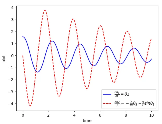
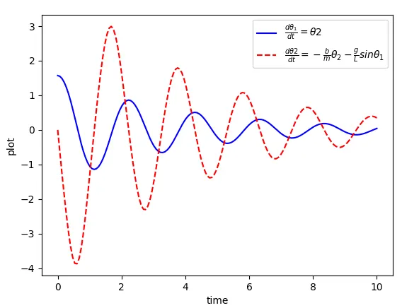
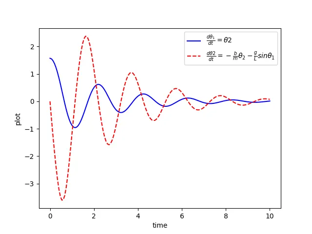
B) Plot different angular displacement and velocity for different damping coefficient :-

1. At b = 0.02 :-

2. At b = 0.05 :-

3. At b = 0.08 :-

4. At b = 0.1 :-

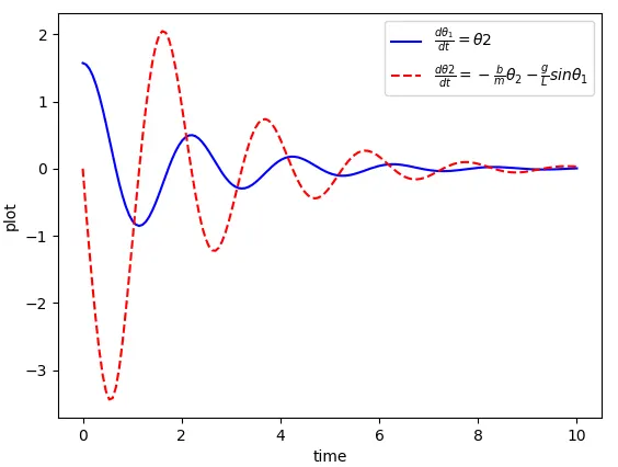
From above figures we can say that as damping coefficient increases the disturbance of angular velocity and angular displacement decreases. Angular displacement starts from 1.8 at zero second and angular velocity starts from zero at zero second.

C. Main python code :-

import numpy as np
from scipy.integrate import odeint
import matplotlib.pyplot as plt
import math
#function that returns dz/dt
def model(theta,t,b,g,l,m):
	theta1 = theta[0]
	theta2 = theta[1]
	dtheta1_dt = theta2
	dtheta2_dt = -(b/m)*theta2 - (g/l)*math.sin(theta1)
	dtheta_dt = [dtheta1_dt, dtheta2_dt]
	return dtheta_dt

b = 0.08
g = 9.81
l = 1
m = 0.1

#install condition
theta_0 = [math.pi/2, 0]

#time points
t = np.linspace(0,10,150)

#solve ODE
theta = odeint(model,theta_0,t,args = (b,g,l,m))
print(theta[:,0])
#plot results
plt.plot(t,theta[:,0],"b-",Label=r"$\frac{d\theta_1}{dt}=\theta2$")
plt.plot(t,theta[:,1],"r--",Label=r"$\frac{d\theta2}{dt}=-\frac{b}{m}\theta_2-\frac{g}{L}sin\theta_1$")
plt.ylabel("plot")
plt.xlabel("time")
plt.legend(loc="best")
plt.show()

D. Animation code :-

import numpy as np
from scipy.integrate import odeint
import matplotlib.pyplot as plt
import math

#function that returns dz/dt
def model(theta,t,b,g,l,m):
	theta1 = theta[0]
	theta2 = theta[1]
	dtheta1_dt = theta2
	dtheta2_dt = -(b/m)*theta2 - (g/l)*math.sin(theta1)
	dtheta_dt = [dtheta1_dt, dtheta2_dt]
	return dtheta_dt

# time array
t = np.linspace(0,20,200)         # 200 .png files in the range of 0 to 10

# inputs
b = 0.05       # damping coefficient
g = 9.81       # gravity
l = 1          # length of the pendulum
m = 0.1        # mass of the ball
ct = 1         # start contour

#initial conditions
theta_0 = [math.pi/2, 0]
x1 = 0
y1 = 0

theta = odeint(model,theta_0,t,args = (b,g,l,m))

for ang in theta[:,0]:              # all the angular displacement and zero angular velocity
	x2 = l*math.sin(ang)
	y2 = -l*math.cos(ang)

	# saveing images in png format
	filename = str(ct) + ".png"
	ct = ct + 1

	# plotting
	plt.figure()
	plt.plot([-1.5,1.5],[0,0],linewidth=8)
	plt.plot([x1,x2],[y1,y2],linewidth=3)
	plt.plot(x2,y2,"o",markersize=15)
	plt.xlim([-1.5,1.5])
	plt.ylim([-1.5,1.5])
	plt.savefig(filename)

E. Animation files :-

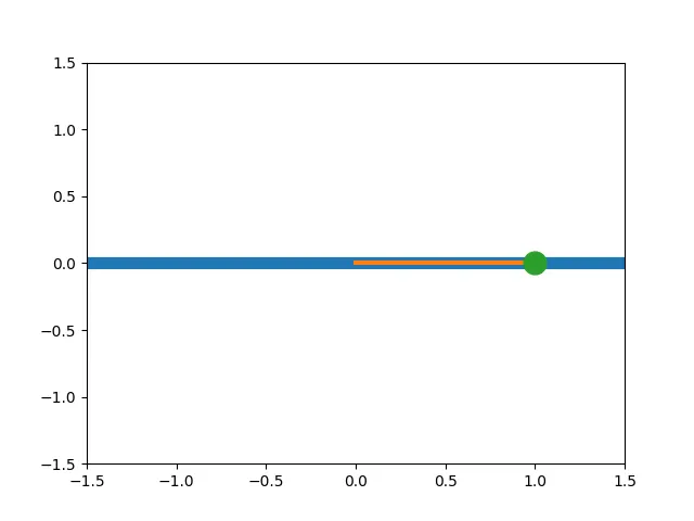
The bob is start from higher velocity and displacement and then decreases as time increases. The bob is rotates very soft way within 180 degree. It starts from 0.011 radian to 1.57 radians.

CONCLUSIONS :-

From above code and animation file we can conclude that-

1. For running this project we must need to install and import numpy, scipy, matplotlib and math module.
2. Define model with all inputs.
3. Due to string motion we must need to define initial and final points.
4. Markersize command is use here for defining sphere size.
5. For loop is use to all the angular displacement and zero angular velocity.
6. Linspace command is use for defining the number of .png files.
7. For any order of png file we need to run the command as “magick %d.png[1-200] output” for converting .png to .gif animation file.

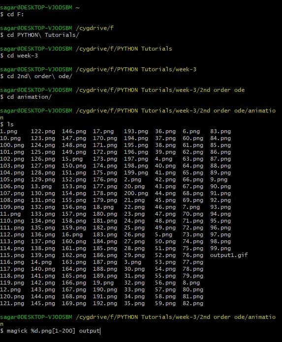
In this way I explain and run here everythings. I write here stepwise explaination of code, facing error while programming and screenshots of those error. This project is very helpful for those who are from mechanical background and they want to go automization industry like robot, spring and stiffness …etc.