Week 3 - Solving second order ODEs

SIMULATION OF SIMPLE PENDULUM BY MATLAB

AIM: The ODE(ordinary differential equation) is used to describe the transient behavior of a system. A simple example is a pendulum.For this pendulum to write a code in MATLAB and simulate the model is the aim.

OBJECTIVE:The objective of this project is to simulate the pendulum in matlab.

INTRODUCTION:

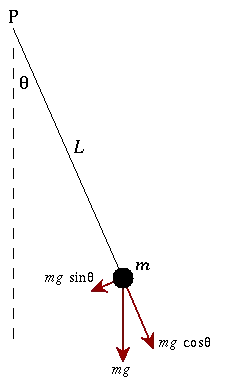
• A simple pendulum consists of a mass m hanging from a string of length L and fixed at a pivot point P. When displaced to an initial angle and released, the pendulum will swing back and forth with periodic motion.

  The differential equation which represents the motion of a simple pendulum is

  
• 

• In the above equation,

  g = gravity in m/s2,

  L = length of the pendulum in m,

  m = mass of the ball in kg,

  b=damping coefficient.

PARAMETERS USED:

• L=1 metre,

  m=1 kg,

  b=0.05.

  g=9.81 m/s2.

  Simulate the motion between 0-20 sec, for angular displacement=0,angular velocity=3 rad/sec at time t=0.

CODE IN MATLAB:

%Program simulating the pendulum motion
clear all
close all
clc

%Input parameters
b=0.05;
L=1;
m=1 ;
g=9.81;

%input conditions
theta=[0;3];
%time points
t_span=linspace(0,20,100);

%ODE fUNCTION
[t,results]=ode45(@(t,theta) ode_func(t,theta,b,g,L,m),t_span,theta);

%ploting
plot(t,results(:,1))
hold on
grid on
title('displacement vs velocity');
plot(t,results(:,2))

%Animation
ct=1;
for i=1:length(t_span)
    x0=0;
    y0=0;
    x1=1*sin(results(i,1));
    y1=-(1*cos(results(i,1)));
    %plotting
    figure(2)
    
  

    plot([x0 x1],[y0 y1],'color','r');
    
    line([-1.5 1.5],[0 0])
    axis([-1.5 1.5,-1.5 1.5]);
    hold on
    plot(x1,y1,'o','color','b');
    hold off
    
    title('simulation of pendulum')
   
    grid on
   
    pause(0.01)
    M(ct)=getframe(gcf);  
    ct=ct+1;         
end
 movie(M);
 videofile=VideoWriter('simple pendulum.avi','uncompressed avi');
 open(videofile);
 writeVideo(videofile,M);
 close(videofile);

EXPLANATION OF THE CODE:

• Above is the code for oscillation of a simple pendulum in MATLAB.
• Input parameters are defined at the beginning of the program.
• Conditions are given to simulate the pendulum,where theta=[0;3].Here in theta we are difining the value for initial conditions as angular displacement is 0;and angular velocity is 3.
• t_span defines the time from 0 to 20 seconds with 100 values.

Ode45:

• A typical approach to solving higher-order ordinary differential equations is to convert them to systems of first-order differential equations, and then solve those systems. The example uses Symbolic Math Toolbox™ to convert a second-order ODE to a system of first-order ODEs. Then it uses the MATLAB solver ode45 to solve the system.
• Define t,theta,b,l,m in another scrip to call the function in main program.
• Second order function is splitted into first oder equations.
• Plot the displacenemt and velocity in the graph.

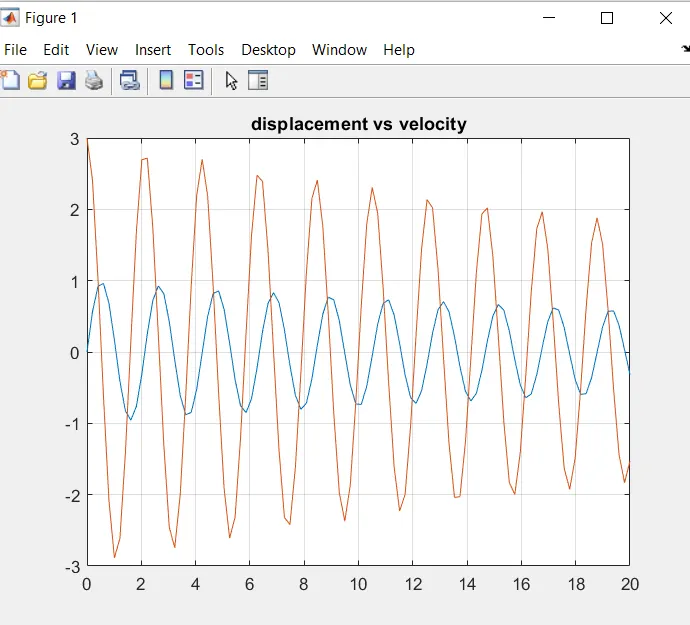
fig:image showing displacement and velocity

ANIMATION:

• To create a animation file we need to use for loop.
• Initial values will be x=0;y=0
• For i=1:length(t_span),which means i takes 100 the values from 0 to 20 seconds
• Now we can define x1 and y1 values.
• Plot them in the graph .
• Now we need to create a circle at x1 and y1 point,to do this we use plot command.
• To animate the plot we are using getframe command under any array say M.
• At the end of the ct is incrementing by one.

SYNTAX FOR MOVIE:

• Movie(M) - plays the N matrix in movie m
• videofile - creates a video file for the movie.
• open(videofile)- opens the movie.
• writeVideo(videofile,M)-Write the video with plot frames in the array M.
• close(videofile)- closes the video file.

CODE FOR FUNCTION:

function [dtheta_dt]=ode_func(t,theta,b,g,L,m)
theta1=theta(1)
theta2=theta(2)
dtheta1_dt=theta2;
dtheta2_dt=-(b/m)*theta2-(g/1)*sin(theta1);
dtheta_dt=[dtheta1_dt;dtheta2_dt];
end

ERRORS:

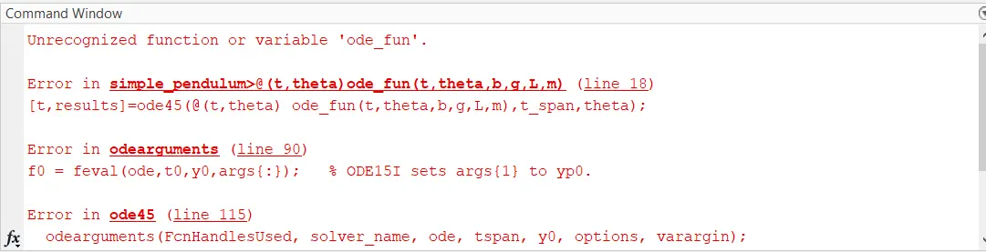
• While calling the function i made a mistake by missing c in ode_func

RESULTS:

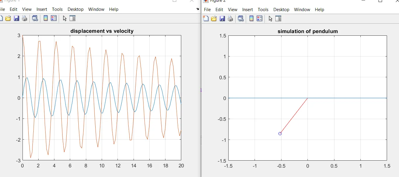
LINK OF THE PROJECT: https://youtu.be/3rgwD3T9We4