Week 3 - Solving second order ODEs

ANALYSIS OF SIMPLE PENDULUM UNDER DAMPED MOTION

AIM:

Analyze the damped motion of simple pendulum using ODE45 solver and code a program to simulate the simple pendulum in matlab.

THEORY:

A simple pendulum consists of object hung by a string from a fixed support. It hangs vertically in its equilibrium position. The object is referred to as the pendulum bob. When the bob is displaced from equilibrium and then released, it begins its back and forth vibration about its fixed equilibrium position. The motion is regular and repeating, an example of periodic motion.

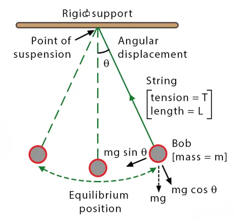
force equations: `mg cos(theta)=T`

`mg sin(theta)= mL(d^2 (theta)/dt^2)``mg sin(theta)= mL((d^2 (theta))/dt^2)`

The restoring force causes the vibrating object to slow down as it moves away from the equilibrium position and to speed up as it approaches the equilibrium position(restoring force is responsible for the vibration). The two forces acting upon a pendulum bob at during the motion. There is the force of gravity that acts downward upon the bob. It results from the Earth's mass attracting the mass of the bob. And there is a tension force acting upward and towards the pivot point of the pendulum. The tension force results from the string pulling upon the bob of the pendulum.

Using ode45 in MATLAB

MATLAB’s standard solver for ordinary differential equations (ODEs) is the function ode45. This function implements a Runge-Kutta method with a variable time step for efficient computation. Ode45 is designed to handle the following general problem:

`(dx)/dt= f(t,x), x(t0) = x0,`

where t is the independent variable, x is a vector of dependent variables to be found and f(t,x) is a function of t and x.

A numerical ODE solver is used as the main tool to solve the ODE’s. The matlab function ode45 will be used & ode45 can only solve a first order ODE. Therefore to solve a higher order ODE, the ODE has to be first converted to a set of first order ODE’s. This is possible since an n order ODE can be converted to a set of n first order ODE’s.

Ode45 is a function in matlab that solves ordinary or partial differential equations using a numerical method.

Typical use of ode45:

[tSol,ySol]=ode45(@(t,y) fName (t,y), [t0, tEnd], y0);

• tSol,ySol: Solution vectors; MATLAB returns ySol for each time tSol.
• fName : Function then returns dy=F(t,y).
• t0, y0 : Initial conditions representing y(t_0)=y_0.
• tEnd : Final value until which the solution is desired.

Syntax: [t ,y] = ode45 (odefun, tspan, y0,options)

Where

tspan = [t0 tf], integrates the system of differential equations y′=f(t,y) from t0 to tf with initial conditions y0.

odefunc(function handle)= The function `dy/dt = odefun(t,y)`, for a scalar t and a column vector y, must return a column vector dydt of data type single double that corresponds to f(t,y). odefun acceptboth input arguments, t and y, even if one of the arguments is not used in the function.

`y_0`(intial cinditions) = Initial conditions, specified as a vector. y0 must be the same length as the vector output of odefun, so that y0 contains an initial condition for each equation defined in odefunc.

options(structure array)= Option structure, specified as a structure array. Use the odeset function to create or modify the options structure.

OBJECTIVES:

1. Analyse the behavior of a pendulum and solve second order ODE equation.
2. Plot a graph of damping motion in pendulum w.r.t time.
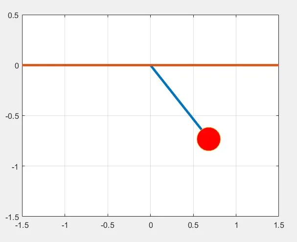
3. Program an animation movie of pendulm motion.

TOOLS USE: Matlab R2020b.

PROCEDURE:

The motion of damped pendulum is given by

`(d^2(theta))/(d(t^2))+b/m*(d(theta))/(d(t))+g/L*sin(theta) = 0`

where

g = gravity = 9.81 m/s2,

L = length of the pendulum = 1m,

m = mass of the ball = 1 kg,

b= 0.05.

Given Assumptions for pendulum motion;

t = 0-20 secs

Initial Angular Displacement = 0,

At t = 0,

Angular velocity = 3 rad/sec.

To define the program ode45 solver is used for solving the ODE, to call the function as 'odefunc', initial parameters are set;

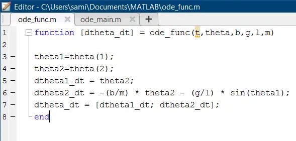
CODE snippet for the above program;

function [dtheta_dt] = ode_func(t,theta,b,g,l,m)

theta1=theta(1);
theta2=theta(2);
dtheta1_dt = theta2;
dtheta2_dt = -(b/m) * theta2 - (g/l) * sin(theta1);
dtheta_dt = [dtheta1_dt; dtheta2_dt];
end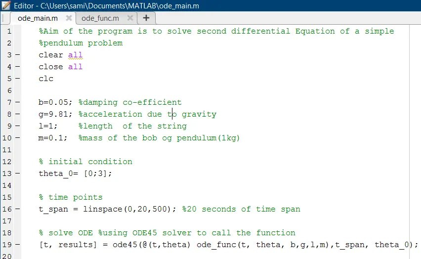

OUTPUT FOR ABOVE PROGRAM,

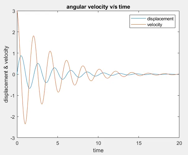
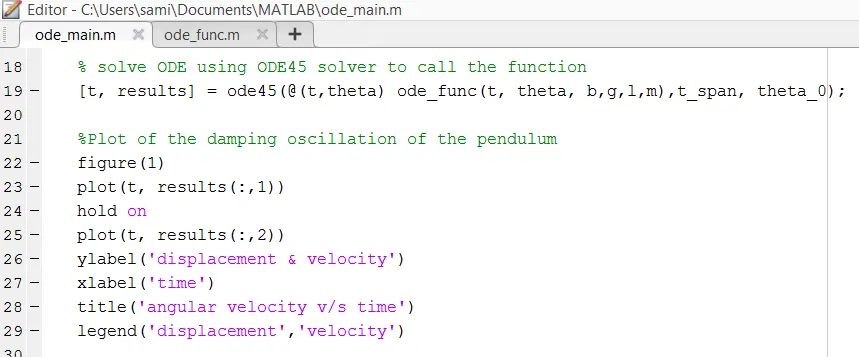
To plot a graph between displacement and velocity, following modifiacations are done to the program,

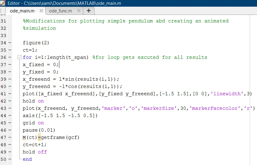
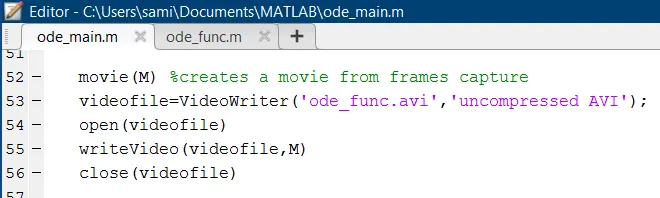
OUTPUT;

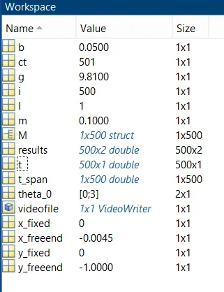
%Aim of the program is to solve second differential Equation of a simple 
%pendulum problem
clear all
close all
clc
 
b=0.05; %damping co-efficient
g=9.81; %acceleration due to gravity
l=1;    %length  of the string
m=0.1;  %mass of the bob og pendulum(1kg)

% initial condition
theta_0= [0;3];

% time points
t_span = linspace(0,20,500); %20 seconds of time span 

% solve ODE using ODE45 solver to call the function
[t, results] = ode45(@(t,theta) ode_func(t, theta, b,g,l,m),t_span, theta_0);

%Plot of the damping oscillation of the pendulum
figure(1)
plot(t, results(:,1))
hold on 
plot(t, results(:,2))
ylabel('displacement & velocity')
xlabel('time')
title('angular velocity v/s time')
legend('displacement','velocity')

%Modifications for plotting simple pendulum abd creating an animated
%simulation

figure(2)
ct=1;
for i=1:length(t_span) %for loop gets excuted for all results 
 x_fixed = 0;
 y_fixed = 0;
 x_freeend = l*sin(results(i,1));
 y_freeend = -l*cos(results(i,1));
 plot([x_fixed x_freeend],[y_fixed y_freeend],[-1.5 1.5],[0 0],'linewidth',3)
 hold on
 plot(x_freeend, y_freeend,'marker','o','markerSize',30,'markerFacecolor','r')
 axis([-1.5 1.5 -1.5 0.5])
 grid on 
 pause(0.01)
 M(ct)=getframe(gcf)
 ct=ct+1;
 hold off
end

movie(M) %creates a movie from frames capture
videofile=VideoWriter('ode_func.avi','uncompressed AVI');
open(videofile)
writeVideo(videofile,M)
close(videofile)

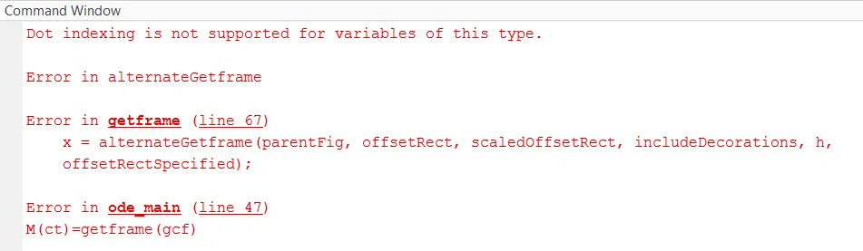
ERROR:

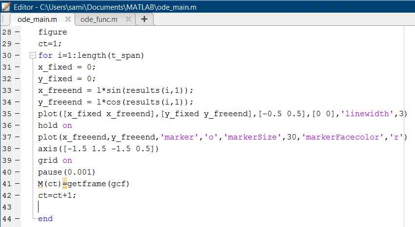
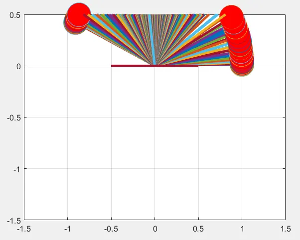
As shown on the below pictures, due to absence of HOLD OFF command. The plot shows different positions of string of pendulum.

If the HOLD ON command is used, the plots at different orientations are saved on a single graphical window.

Both HOLD ON and HOLD OFF commands must be used to avoid the mis-positions.

In order of fix the error, the freeend of y-axis should be at negative y-axis.

y_freeend = -l*cos(results(i,1));

The link to the animation of simple pendulum is,

https://youtu.be/V0BFHTlz2B8

CONCLUSION:

MATLAB is a computer program that provides the user with a convenient environment for performing many types of calculations. The case study shows that dealing with differential equations of the mathematical models of engineering systems mostly encounter difficulties in term of the MATLAB programming. The major restriction of the MATLAB solve code is that the system of differential equations should be organized in the form of the first order differential equations, whereas the core engineering application either in the form of second order or in even mixed order. Therefore, transformation of the system of differential equations is mandatory, and this can make mistakes beside to the time spent.

References:

• Research paper Using MATLAB/ode45 for Solving Differential Equations in Engineering Applications by Waleed K. Ahmed .
• Matlab and its Applications in engineering, by Raj bansal.