Week 3 - Solving second order ODEs

Solving a 2nd Order Diffrential Equation to find the Transient Behaviour of a Simple Pendulum using Python

Aim:

* To solve a 2nd order diffrential equation, so that we can find the transient behaviour of a simple pendulum for its given input conditions for displacement and velocity over a given time period.

* To make a animation of the given simple pendulum's motion using python coding.

* To visualize the behaviour of the pendulum by plotting the displacement curve and velocity curve over the given time period.

Procedure:

* Ordinary diffrential equation is a very important phenomenon which when solved, can give a lot of engineering factors.

* The second order ODE has independent variables and dependent variables. This equation mainly gives the relation between the independent and dependent variable, by intergrating them and with this relation we can solve many important phenomenon.

* The main idea to solve a 2nd order ODE is by breaking them into two individual first order ODE.

* The given second order ODE is,

d^2 * (theta) / (dt) ^ 2 + (b/m) * d(theta) / dt) + (g/L) * sin(theta) = 0

* if we solve this equation for a simple pendulum we can figure out the angle of the pendulum changing with respect to time and we can find the angular displacement and angular velocities with respect to time.

* Same equation can also be used to measure the transient behaviour of a suspension system of an automobile and by seeing the displacement and velocity curves, we can analyze for the adequate damping needed for that suspension system to reduce the shocks.

* The equation is solved using the python using and ordinary diffrential equation solver to Simulate the motion between 0-20 sec, for angular displacement=0, angular velocity=3 rad/sec at time t=0 and for the given input data

* Then by stiching all the plots generated through the python program, we are creating an animation of the simple pendulums motion.

Input Parameters:

* The initial condition of the simple pendulum and its input parameters are specified below,

1. Initial distance travelled by the bob = 0

2. Initial angular velocity given to the bob = 3 rad/sec

3. Time span = 20 seconds (with 200 time step)

4. Gravity (g) = 9.81 m/s^2

5. Length of the pendulum (l) = 1 m

6. Mass of the bob (m) = 1 kg

7. Damping coefficient (b) = 0.05

* Then with all of these values we can bring the transient motion of the simple pendulum using the python program as below.

Python Coding:

import math
import numpy as np
import matplotlib.pyplot as plt
from scipy.integrate import odeint

# function program that returns dtheta/dt

def model(theta,t,b,g,l,m):
	theta1 = theta[0]
	theta2 = theta[1]
	dtheta1_dt = theta2
	dtheta2_dt = -(b/m)*theta2 - (g/l)*math.sin(theta1)
	dtheta_dt = [dtheta1_dt,dtheta2_dt]
	return dtheta_dt

# input parameters
# Damping coefficient
b=0.05
# Centre of gravity
g=9.81
# Mass of the bob
m=1
# length of the bob
l=1

# Initial condition for displacement and velocity
theta_0 = [0,3]

# Time values
t = np.linspace(0,20,200)

# Solving the ode function
theta = odeint(model,theta_0,t,args=(b,g,l,m))	

# Plotting
plt.plot(t,theta[:,0],'b-',label=r'$\frac{d\theta_1}{dt}=\theta2$')
plt.plot(t,theta[:,1],'r--',label=r'$\frac{d\theta2}{dt}=-\frac{b}{m}\theta_2-\frac{g}{l}sin\theta_1$')
plt.xlabel('Time (sec)')
plt.ylabel('Angular displacement & Angular velocity')
plt.title('Angular displacement & Angular velocity vs Time of a simple pendulum')
plt.legend(loc='best')
plt.show()

#creating the simple pendulum animation
x0=0
y0=0
ct=1 
for i in  theta[:,0]:
	x1=l*math.sin(i)
	y1=-l*math.cos(i)
# Generating the individual figures
	filename = 'test%05d.png' % ct
	ct=ct+1
	plt.figure()
	# creating the fixed line
	plt.plot([-2,2],[0,0])
	# creating the bob string
	plt.plot([x0,x1],[y0,y1])
	# creating the bob
	plt.plot(x1,y1,'o',markersize = 10)
	plt.xlim([-2,2])
	plt.ylim([-2,2])
	plt.savefig(filename)

* First we are importing all the required libraries for executing the code, especially the 'scipy' module which has the ordinary diffrential equation solver in it.

* Then we pass on all the input parameters of the simple pendulum like, gravity, mass and length of the pendulum and damping coefficient.

* Then we are giving the time span of the simple pendulum's oscillation as 20seconds using linspace command to select 200 step between 0 & 20 seconds.

* For simple construction of the program we are creating a function called 'model' , then we can call this function into to program where ever required.

* Then in the function program, we specify θ1 and θ2 and then by passing all the input arguments we are calculating the values of both the splitted first order ODE'S (i.e) dθ1 / dt & dθ2 / dt.

* Giving all the input values, we can solve this equation of a simple pendulum to return the values of dθ/dt

* Then we are using 'odeint' solver to solve the systems of diffrential equations with the Initial conditions given in theta_0, time span, dθ/dt value from the function program and passing all the input arguments.

* The 'odeint' solver integrates the system of differential equations throught the whole time span starting from 0 seconds to 20 seconds (with 200 inbetween points), with the initial conditions specified in 'theta_0' and then gives the Result 'Theta'. Each row in the result array corresponds to a time span, thus giving the results for Angular dispacement & Angular velocites with respect to the time.

* Finally we plot the results to visualize the angular displacement and velocities with respect to time. The result 'theta' has two coloumn and 200 rows. The first column gives the displacement values and the second column gives the velocity values and we plot them correspondingly with respect to the time array.

* Then the simple pendulum is made using plot command. The base reference line is made, then bob string and bob is made using plot commands.

* The bob movement is predicted using a 'For loop' where the vertical and horizontal coordinates are integrated for all the displacement values from the result.

* Then we find all the plots are getting saved in a single figure window and so to rectify this we are using, 'plt.figure' command so that we save all the output figure in individual figure window.

* To save the figure in order from 1 to 200 we are using a counter variable (ct) in the for loop and then we are assigning this to a variable called 'filename'.

* This filename is used while saving the individual figures and as it is under the for loop, the filename from '1 to 200.png' is generated for all the output figures accordingly.

* Then all the generated plots are saved in a folder and then it is used to create a animation to visualize the transient movement of the simple pendulum.

* A program called 'Imagemagick' is used to create a gif file out of the generated plots using the command promt window.

Result:

*The python codes were done to visualize the transient behaviour of a simple pendulum for the given input conditions and is given below,

(i) The Angular velocity and displacement vs Time with damping coefficient (b= 0.05):

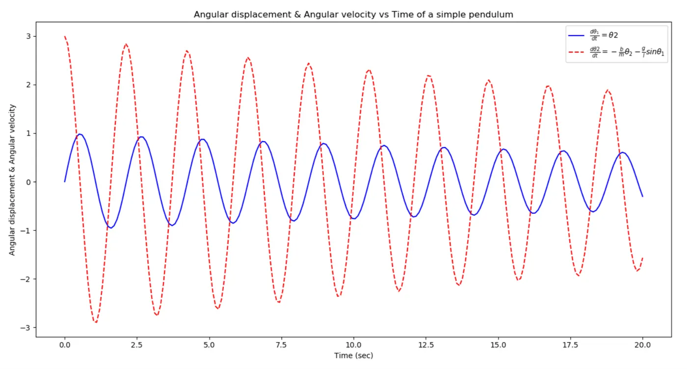
* Here we can see the movement of the simple pendulum's bob with repect to time. The blue line shows the Angular displacement with respect to time and the dotted Red line shows the Angular velocity with repesct to time.

* The angular displacement starts from 0 and it goes to a maximum distance of 1 m on both the forward and backward axis and at the end of the time period the movement is reduced.

* The angular velocity starts from 3 rad/sec initially and it goes on decresing with increase in time and at the end of the time period of 20 seconds the velocity of the pendulum's motion is 2 rad/sec and it goes on decresing with time.

(ii) The Angular velocity and displacement vs Time with damping coefficient (b= 0.2):

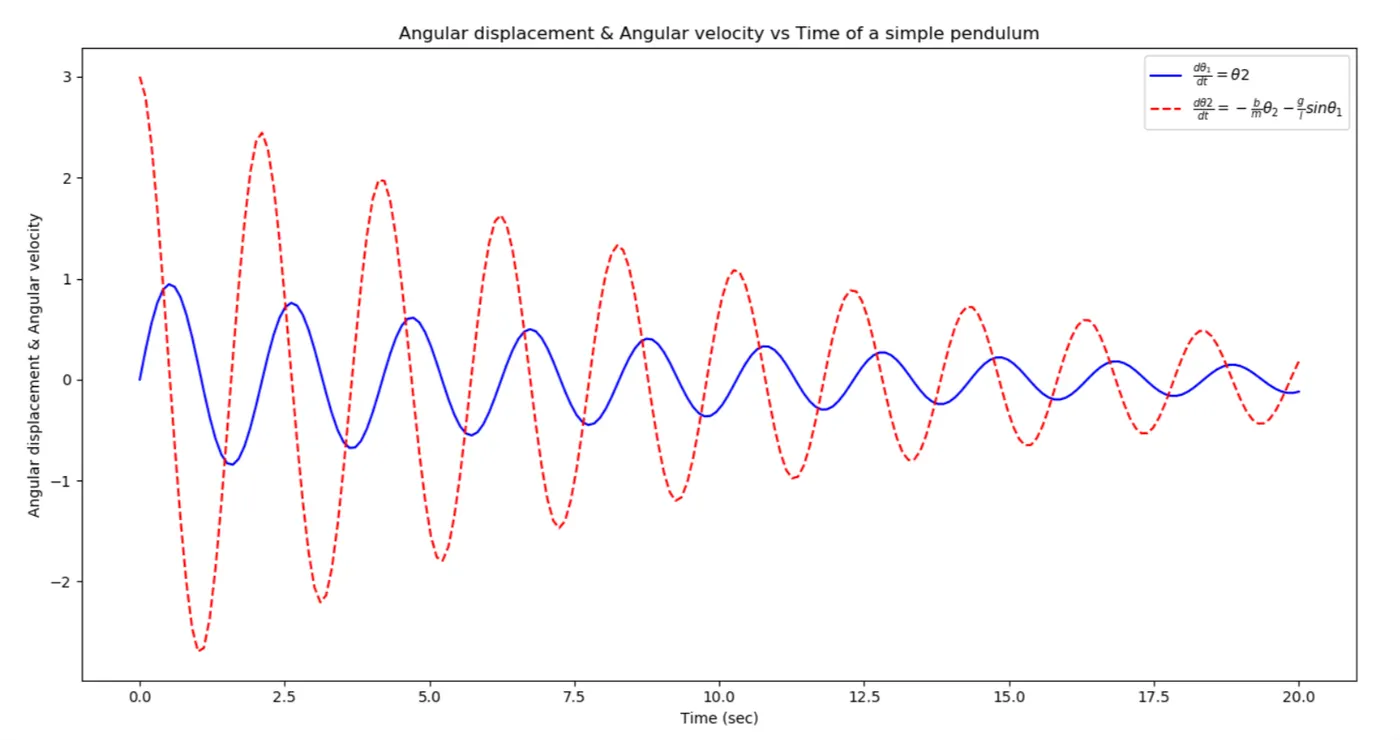
* Here we have increased the damping coefficinet by four times and we see the movement of the simple pendulum's bob with repect to time. The blue line shows the Angular displacement with respect to time and the dotted Red line shows the Angular velocity with repesct to time.

* The angular displacement starts from 0 and it goes to a maximum distance of 1 m on both the forward and backward axis and at the end of the time period the movement is reduced.

* The angular velocity starts from 3 rad/sec initially and it goes on decresing with increase in time and at the end of the time period of 20 seconds the velocity of the pendulum's motion is 0.5 rad/sec and it goes on decresing with time.

* Compared to the previous case, here the movement and velocity is getting arrested quickly with four times increase in damping coefficient (b). By changing the inputs as per our desire we can find out the angular displacement and velocity with respect to time (i.e) in case f a simple pendulum, how quick the oscillations can be damped, can be analysed and a balanced output can be determined from this python program.

* Similarly this 2nd order ordinary diffrential equation can also be used to study the shock absorbing capacity of a newly developed spring suspension of a vehicle. By providing all the adequate data for mass and damping coefficient of our design we can check for its capacity of absorbing the shocks and how well the vibrations are getting damped.

* Having this knowledge, we can develope the balanced spring suspension for a vehicle with this python program of solving the 2nd order diffrential equation system.

Transient motion of the Simple Pendulum:

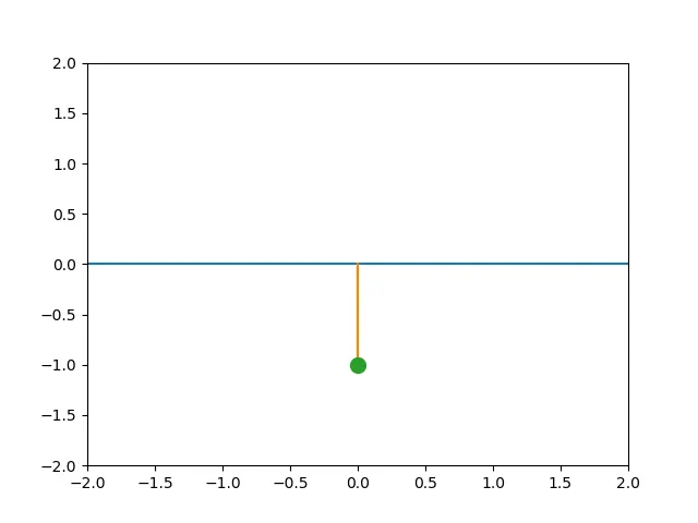
* The above animation shows the transient motion of the simple pendulum for the gven time period.

* The simple pendulum's motion is thus visualized for the given input conditions of displacement and velocity with the given input parameters for the mass, gravity and damping coefficient of the simple pendulum, with this python program.

* Same 2nd order ode equation, can also be used to measure the transient behaviour of a suspension system of an automobile. By seeing the Angular displacement and velocity curves with respect to time, we can analyze for the adequate damping needed for a balanced suspension system to reduce the shocks.