Week 3 - Solving second order ODEs

Aim:

To Solve the Second Order Ordinary Differential Equation (ODE) & to simulate with an example of Simple Pendulum

Description:

• Newton’s Second Law: In an inertial frame of reference, the vector sum of the forces F on an object is equal to the mass m of that object multiplied by the acceleration an of the object:

F = ma

• Example: The trajectory of a projectile launched from a cannon follows a curve determined by an ordinary differential equation that is derived from Newton's second law.

• ODE: In mathematics, an ordinary differential equation(ODE) is a differential equation containing one or more functions of one independent variable and the derivatives of those functions.

The motion of Simple Pendulum by Second order ODE

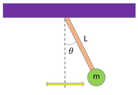
`(d^2θ)/ dt^2 + b/m (( dθ)/ dt ) + g/L sin θ = 0`

Where,

`theta`= Angular Displacement

t = Time (s)

b = Damping Coefficient

m = Mass of Ball (Kg)

L = Length of String (m)

g = Gravity

By solving Second Order ODE, we will get positions of the pendulum as a function of time.

`(d^2θ)/ dt^2 + b/m (( dθ)/ dt ) + g/L sin θ = 0`

Let’s consider,

`θ= θ_1`

Differentiate ODE w.r.t. time to get order one equation.

• 1^st order ODE of Angular Displacement.

`(dθ)/dt=(dθ_1)/dt= θ_2`

Substituting in 2^nd Order ODE, we get

`(d^2 θ)/(dt^2 )=(d^2 θ_1)/(dt^2 )=d/dt ((dθ_1)/dt)=(dθ_2)/dt`

• 1^st order ODE of Angular Velocity.

`(dθ_(2 ))/dt=- b/m (θ_(2 ))- g/L sin(θ_1)`

Python Code to solve & simulate 2nd Order ODE with Sample Pendulum as an example.

# Importing important modules

import numpy as np
from scipy.integrate import odeint
import matplotlib.pyplot as plt
import math

# Functions that returns dz/dt:

def model(theta,t,b,g,l,m):

	theta1 = theta[0]
	theta2 = theta[1]

	dtheta1_dt = theta2
	dtheta2_dt = -(b/m)*theta2 - (g/l)*math.sin(theta1)
	
	dtheta_dt = [dtheta1_dt, dtheta2_dt]
	return dtheta_dt


b = 0.05
g = 9.81
l = 1
m = 1

# Initial condition

theta_0 = [0,3]

# Time points
t = np.linspace(0,20,150)

# solve ODE
# odient function from Scipy module. It is a function that integrates systems of differential equations.

theta = odeint(model,theta_0,t, args =(b,g,l,m))

# Plot results

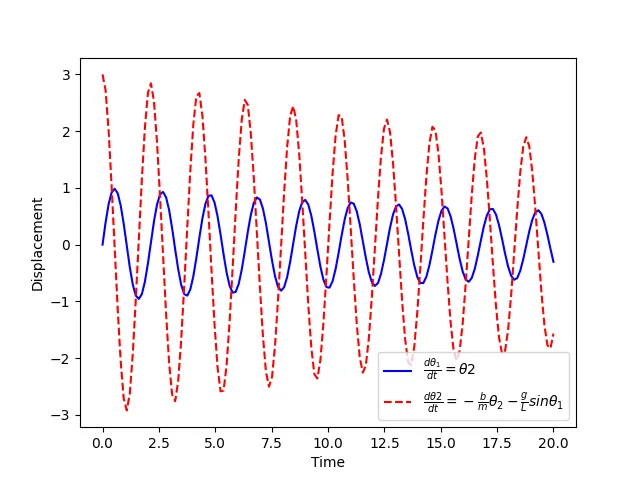
plt.plot(t,theta[:,0],'b-',Label = r'$\frac{d\theta_1}{dt}=\theta2$')
plt.plot(t,theta[:,1],'r--',Label = r'$\frac{d\theta2}{dt}=-\frac{b}{m}\theta_2-\frac{g}{L}sin\theta_1$')

plt.ylabel('Displacement')
plt.xlabel('Time')
plt.legend()
plt.show()

# Counter

ct = 1

for t1 in theta[:,0]:
	# initial Co-ordinates for fixed point
	x0 = 0
	y0 = 0

	# End Co-ordinates for string
	x1 = l* math.sin(t1)
	y1 = -l* math.cos(t1)

	filename = str(ct) + '.png'

	ct = ct + 1

	plt.figure()

	# Plotting Horizontal line

	plt.plot([-0.5, 0.5],[0, 0], 'g', linewidth = 5)

	# Plotting String of Pendulum
	plt.plot([x0, x1], [y0, y1], 'r')

	# Plotting Ball of Pendulum
	plt.plot(x1, y1, 'o',markersize = 30)

	# Limiting X - axis
	plt.xlim([-1.5, 1.5])

	# Limiting Y- axis
	plt.ylim([-1.5, 1.5])

	# Title
	plt.title('Simple Pendulum Animation using Python')

	plt.savefig(filename)

Result:

Output Animation link : https://youtu.be/eK6A-RHI2hU

References:

• https://en.wikipedia.org/wiki/Ordinary_differential_equation#Solutions