Week 3 - Solving second order ODEs

Python code to describe the transient behavior of a Simple pendulum with a damping constant of 'b'.

Theory

In Engineering, ODE is used to describe the transient behavior of a system. A simple example is a pendulum

The way the pendulum moves depends on Newton's second law. When this law is written down, we get a second order Ordinary Differential Equation that describes the position of the "ball" w.r.t time.

The following Ordinary Differential Equation describes the motion of a simple pendulum with a damping constant b">bb.

In the above equation,

g = gravity in m/s2,

L = length of the pendulum in m,

m = mass of the ball in kg,

b=damping coefficient.

Parameters for the simulation.

L=1 metre,

m=1 kg,

b=0.05.

g=9.81 m/s2.

Time period of the motion = 0-20 sec, for angular displacement=0,angular velocity=3 rad/sec2 at time t=0.

The following python code gives us the motion of a simple pendulum with the given parameters.

"""
	Python code to describe the transient behavior of a Simple pendulum with a damping constant of 'b'.
	by Saurabh Nambiar 
"""

# Importing Libraries
import matplotlib.pyplot as plt
import math
import numpy as np
from scipy.integrate import odeint

 
# Defining function that returns theta array/list
def model(theta,t,b,g,l,m):
	theta1 = theta[0]
	theta2 = theta[1]
	dtheta1_dt = theta2
	dtheta2_dt = -(b/m)*theta2 - (g/l)*math.sin(theta1)
	dtheta_dt = [dtheta1_dt, dtheta2_dt]
	return dtheta_dt

# Inputs
b =0.05
g = 9.81
l = 1
m = 1

# Initial Conditions
theta_0 = [0, 3]

# Time Points
t = np.linspace(0,20,150)

# Solve ODE
theta = odeint(model,theta_0,t,args = (b,g,l,m))




# Creating a combined plot of Velocity and displacement
plt.plot(t,theta[:,0],'b-',label=r'Displacement (m)')
plt.plot(t,theta[:,1],'r--',label=r'Velocity (m/s)')
plt.legend()
plt.xlabel('Time')
plt.ylabel('Magnitude of Displacement and Velocity')
plt.savefig('D and V plot')
plt.show()

# Creating Plots for animation of Pendulum using for loop
ct = 1
for i in theta[:,0]:
	x_start = 0
	y_start = 0

	x_end = l*math.sin(i)
	y_end = -l*math.cos(i)

	filename = 'test%05d.png'% ct
	ct = ct + 1

	plt.figure()
	# Plotting the base of pendulum
	plt.plot([-1, 1],[0, 0],linewidth=3,color='black')
	# Plotting the string
	plt.plot([x_start,x_end],[y_start,y_end],linewidth = 3,color='blue')
	# Plotting the bob
	plt.plot(x_end,y_end,marker='o',markersize = 20, color='red')
	plt.ylim([-1.25,0.25])
	plt.savefig(filename)

Results.

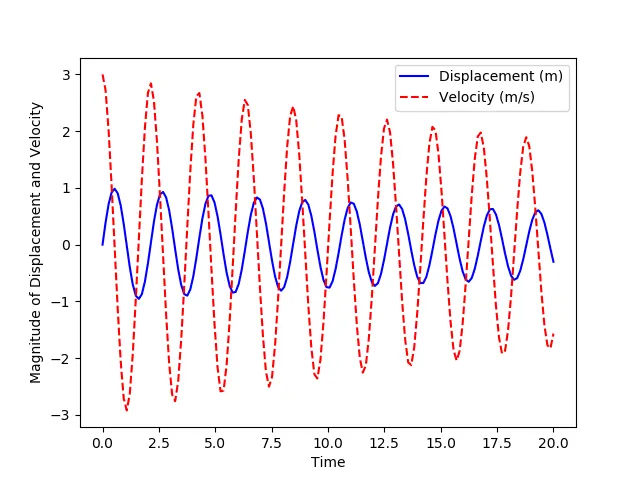
1. Displacement and Velocity Plot.

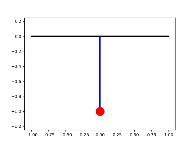
2. Plotting the Pendulum.

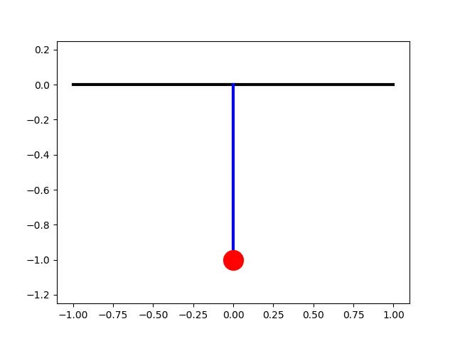
YouTube Link for the output of the given code

Observations.

It is observed that over the time span of 20 seconds the amplitude of the motion of the pendulum decreases, this is due to the damping factor. If we increase this factor the pendulum will come to rest faster. The damping factor is like a frictional force that acts opposite to the motion of the pendulum bob. (Use the link in the blue text to watch the pendulum simulation it was generated using ezgif.com).