Solving Second Order Differential Equations in MATLAB

Project Title:- Solving 2nd Order Differential Equations using MATLAB program.

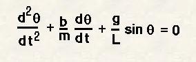
Introduction:- ODE's are very important in engineering and they describe a lot of important phenomena and by solving these ODE's we can understand the systems.

A couple of examples are:-

1. Simple Pendulum
2. Damper, Spring & Mass system

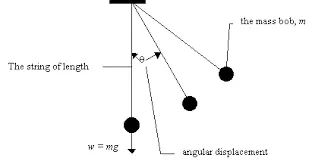
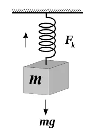
General Solving of 2nd Order Differential Equations:-

2nd ODE:-

• In order to solve the 2nd ODE's or any higher ODE's, we need to break them into 1st ODE.

Assume:-

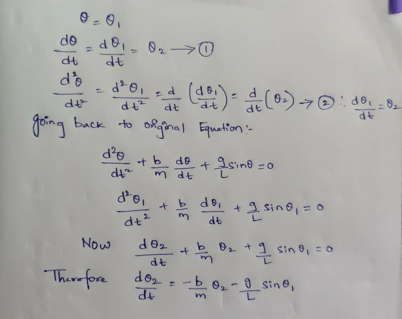
Now Coming to MATLAB:-

For solving ODE for a Simple Pendulum using the above equation in general:-

• A function needs to be defined.
• ODE45 is an inbuilt function in Matlab
• There are 2 ODE's that need to be solved. Displacement & Velocity
• with respect to the equation below code needs to be executed.
• dtheta_dt is defined as a column matrix

function [dtheta_dt] = ode_func(t, theta, b, g, l, m)

theta1 = theta(1)
theta2 = theta(2)
dtheta1_dt = theta2;
dtheta2_dt = -(b/m)*theta2 - (g/l)*sin(theta1);
dtheta_dt = [dtheta1_dt; dtheta2_dt];
end

• Now that the function is defined which I used to solve the below program for given Inpedendant Parameters.
• b - Damping Coefficient
• g - Gravity
• l - Lenth of Pendulum
• m - Mass

clear all
close all
clc

b = 0.01;
g = 9.81;
l = 1;
m = 1;

theta_0 = [0; 5];
t_span = linspace(0,10,500);

[t, results] = ode45(@(t, theta) ode_func(t,theta,b,g,l,m),t_span,theta_0);
plot(t, results(:,1))
hold on
plot(t,results(:,2))
xlabel('time')
ylabel('plot')

• ode45 (t, theta) is defined by the function; ode_func & the independent parameters stated above
• Time & Results are obtained and of the column vector.

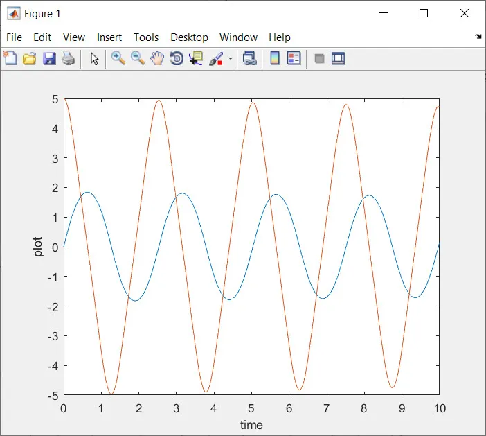
Plotting for Displacement & Velocity:-

1. Blue refers to Displacement as it starts from 0
2. Red refers to Velocity which starts at 5 m/s

To write a program for the parameters below:-

• L=1 metre; L = length of the pendulum in m,
• g=9.81 m/s^2; g = gravity in m/^2,
• m=1 kg; m = mass of the ball in kg,
• b=0.05; b=damping coefficient.
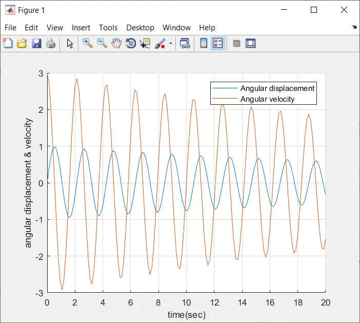
• Simulating the motion between 0-20 sec, for angular displacement=0,angular velocity=3 rad/sec at time t=0.

% 2nd ODE
clear all
close all
clc
b = 0.05   % Damping coefficient
g = 9.81   % Gravity (m/s^2)
l = 1      % Length of penndulum
m = 1      % Mass of the pendulum (kg)

% Initial conditions
% Angular displacement = 0 and Angular velocity = 3
theta = [0; 3] 
% Time length
t_span = linspace(0,20,150)

% ODE function
[t, results] = ode45(@(t, theta) ode_func(t,theta,b,g,l,m),t_span,theta);

% Graph plotting
figure(1)
hold on 
plot(t,results(:,1))
plot(t,results(:,2))
xlabel('time(sec)')
ylabel ('angular displacement & velocity')
legend('Angular displacement','Angular velocity')
grid on

figure(2)
hold on
x0 = 0
y0 = 0
ct = 1

% Pendulum movement using for loop

for i = 1:length(t)
  x1 = l*sin(results(i,1))
  y1 = -l*cos(results(i,1))
   
plot([x0,x1],[y0,y1],'color','b', 'linewidth', 5)
hold on
plot([-1.5,1.5],[0,0],'linewidth',5)
hold on
plot(x1,y1,'o', 'markersize',15, 'markerfacecolor','r')

axis([-1.5 1.5 -1.5 1.5])
grid on
hold off

pause (0.05)
M(ct)= getframe(gcf);
ct = ct + 1;
end

% Creating the animation

movie(M)
videofile = VideoWriter('Pendulum.avi', 'uncompressed avi');
open(videofile)
writeVideo(videofile,M)
close(videofile)

Plotting:-

Animation of Simple Pendulum:-

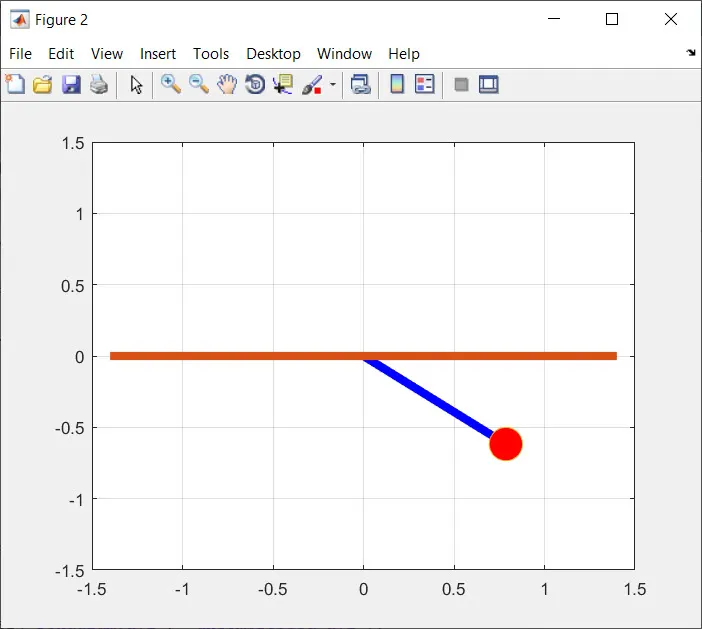
Animation Link:- https://drive.google.com/file/d/1jz8bYqGIicHp-Tt-ovghrpQig-WIFItd/view?usp=sharing