Week 3 - Solving second order ODEs

Objective: To solve the second order ODE that defines the motion of a simple pendulum with damping, and to simulate the motion

Theory: The motion of a simple pendulum with damping is defined by the following governing equation:

`(d^2 θ)/(dt^2 )+b/m (dθ)/dt+g/l sinθ=0`

where `theta` = angular displacement

b = damping co-efficient

m = mass of the pendulum

l = length of the pendulum

g = accelration due to gravity

We will use Runge-Kutta method to solve this equation to find various values of `theta` and `omega` at given values of time t.

For that we will have to convert it to a first order ODE.

we do that by taking `θ=θ_1` , `(dθ_1)/dt = theta_2` and substituting it in the equation. It then reduces to the following first order equation:

`(dθ_2)/dt+b/m θ_2+g/l sinθ_1=0`

After arranging it so that we have

`(dθ_2)/dt=-b/m θ_2-g/l sinθ_1`

Note that if we integrate `theta_2` we get angular displacement, and if we integrate `(dθ_2)/dt` we get the angular velocity, which are the results we are interested in.

This is exactly what we will do using RK4 method. The ode45 function in MATLAB uses the RK4 algorithm to solve a first order ODE and get the results for a given time span and initial conditions

By arranging the two equations in matrix form we get the following

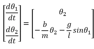
It can be reorganised into

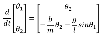
The LHS matrix is the solution matrix which defines our variable.

We can simply call it `θ`

We need to solve the RHS using RK4 method in order to simulate the simple damped pendulum

Code:

A. Function to create an output array of the RHS matrix for the ode45 function:

We have to create a custom function that defines the terms in the RHS matrix and output them when called.

function[result] = ode_pendulum(t,theta,b,g,l,m)

%defining the terms in the solution matrix (LHS of y'=f(x))
theta1 = theta(1); %theta1 is angular position
theta2 = theta(2); %theta2 is angular velocity

%defining terms in the RHS which needs to be solved
c = theta2;
v = (-b/m)*theta2-(g/l)*sin(theta1);
result = [c;v];
end

Explanation:

The function will use t, theta,b,g,l and m, which are part of the terms in the result matrix

Here we are defining the two terms in the solution matrix theta.

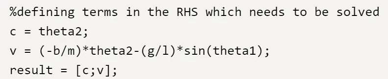
Here we define the terms in the RHS matrix as per the theory and create the output result as a matrix of those two terms.

This output will be used by the ode45 function to solve the equation and find out the values of theta1 and theta2 for various values of t.

B. Main program to solve the differential equation:

Here we will use the above defined function to get the input for the ode45 function

clear all
close all
clc

%setup
tspan = linspace(0,20,500); %number of time integrals over which the various values of displacement and velocity will be calculated
theta_0 = [0;3]; %initial values of displacement and velocity

b = 0.05; %damping co-efficient
m = 0.1; %mass
g = 9.81; %acceleration due to gravity
l = 0.30; %length of pendulum

[t,results] = ode45(@(t,theta) ode_pendulum(t,theta,b,g,l,m) ,tspan,theta_0); %ode function to get solve the function output of ode_pendulum

%Fixed end of pendulum
x0 = 0;
y0 = 0;

%For loop to plot the moving end of pendulum
for i=1:length(tspan)
    thetax = results(i,1); %thetax is the instantaneous angle made by the pendulum with the vertical
    x1 = l*sin(results(i,1)); %x co-ordinate of the moving end
    y1 = -l*cos(results(i,1)); %y co-ordinate of the moving end
    plot([-0.075,0.075],[0,0],'linewidth',3,'color','black');
    hold on;
    plot([x0,x1],[y0,y1],'color','b'); %plotting the pendulum
    plot(x1,y1, '-o','MarkerSize',15,'MarkerEdgeColor','black','MarkerFaceColor','r') %plotting the marker
    hold off;
    axis([-0.25,0.25,-0.4,0.1]); %setting axes
    M(i)=getframe(gcf); %storing the current figure frames in the M array
end

%Generating a movie from the stored frames
movie(M);
file = VideoWriter('pendulum.avi');
open(file);
writeVideo(file,M);
close(file);

Explanation:

1. We start by setting up the inputs and choosing the timespan:

2. Next we use the ode45 function to solve the output of the ode_pendulum function we defined

In this case theta is the 2x1 solution matrix, and the output from ode_pendulum is a function of that matrix.

ode45 will solve the funcion using RK4 numerical method, using the initial condition theta_0 and the timespan tspan.

The result matrix contains two columns, displacement and velocity at various values of t.

3. Now we plot the displacement against time:

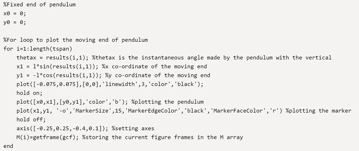
Here we keep one end of the pendulum at 0,0 and the other end is defined by the instantaneous x and y co-ordinates of the displacement.

we define thetax as the instantaneous angle made by the pendulum with the vertical

Then we define x1 and y1, which are the co-ordinates of the movin end, as functions of l and thetax.

We plot a fixed line that acts as the support for the fixed end of the pendulum, for animation purposes.

Then we plot the pendulum movement using a for loop that iterates from 1 to length(tspan)

Thus we are plotting a line from 0,0 to the endpoint for every tspan value.

The figure frames are saved in the M array and used to create a video file as shown:

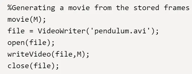
Thus we have solved the governing ODE of a simple damped pendulum for the displacement and velocity, and animated the motion.

Output:

Errors and Fixes:

1.

Error:

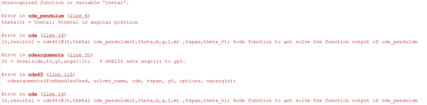
This error occured because we used a matrix index on the LHS while the variable on the RHS as shown:

theta1 and theta2 should form the LHS and the matrix indices should be on the RHS as shown below:

The above change fixed the errors