Week 3 - Solving second order ODEs

The code given below will give us a plot of displacement & velocity of the bob of a simple pandulum as its motion comes to rest under the action of gravity with respect to time. It also gives us the animation of the actual motion of the pendulum as it damps.

clear all
close all
clc

%% INPUTS
%to define the variables as dampening ratio, Gravitational acceleration,
% Mass of the bob, & length of the thread
b = 0.05;
g = 9.81;
m = 1;
l = 1;

% Initial values of displacement & velocity
theta_0 = [0;3];

% time span that gives 500 values between 0 & 10 seconds
t_span = linspace(0,20,500);

%% Computation 
%ODE Solver which gives value of 'results' i.e velocity & displacement for each value of time 't'
[t, results] = ode45(@(t,theta) ode_func(t,theta,b,g,l,m),t_span, theta_0);

%% Plotting 
% To plot the graph to depict the dampening of the bob as velocity  & Displacement gradually become zero 
figure(1)
% To index the first column of results vector for plotting time vs displacement
plot(t,results(:,1))
hold on 
% To index the second column of results vector for plotting time vs velocity
plot(t,results(:,2),'color','r')
ylabel('plot')
xlabel('time')
%% Animation
% first we declare the counter to be 1 
ct = 1
% for the length of timespan we repeat the following plotting command
for i = 1:length(t_span)
   THETA1(i) = results(i,1);
x0 = 0;
y0 = 0;

y1 = -l*cos(THETA1(i));
x1 = l*sin(THETA1(i));

%plotting
figure(2)
plot([x0 x1],[y0 y1],'linewidth',3);
axis([-2 2 -1.5 0.5]);
hold on
plot(x1,y1,'marker','O','markersize',15,'markerfacecolor','r');
pause(0.01)
hold off
M(ct)= getframe(gcf);
ct = ct+1

end

%% Movie generation 
movie(M)
videofile = VideoWriter('pendulum motion.avi','Uncompressed AVI')
open(videofile)
writeVideo(videofile,M)
close(videofile)
%% End

• First we use, ‘clear all’, ‘close all’ & ‘clc’ commands to clear/delete the previously stored variables, close all previous command windows & figures, & clear the command window, respectively. Then we declare the variables to be used such as the damping coefficient, gravitational acceleration, Mass of the bob, & length of the pendulum.

In the variable theta_0 we are storing the initial values of position & velocity of the bob at the initial point as a matrix of 1 X 2. Thus the initial displacement of the pendulum is 0, & the initial angular velocity is 5 rad/s.

Then to define the value for time over which the values of displacement & velocity are to be integrated. We use variable ‘t_span’ an array which goes from 0-10 seconds with 500 values in between.

Now to solve the ODE equation we use one of the in-built solver in MATLAB, ode45 solver.

Ode45 gives the solution vectors for results (displacement & velocity) for each value of t (time) during t_span.

The Syntax of ode45 is as follows- 

1. We declare that its main inputs are t & theta this is called the anonymous as it stores the values of the previous (n-1)^th value  which were calculated in the previous case when the Objective function (ode_func) was executed.
2. Then we declare the objective function (ode_func) which defines the relation between time & results.
3. Then we declare the range(t_span) of independent variable(t) for which the values of results are to be integrated.
4. Then we declare the initial value of results. (theta_0).

As the output now we get results as a matrix of 500 rows and 2 columns.(Figure.1)

Now we declare figure (1) in the code in which we plot the graph for the curves of displacement & velocity.

Since the first curve is of displacement which is given by the first column of the results vector to plot the curve for displacement vs time we use the plot command & index the first column only.

Similarly, for the velocity vs time curve we index the second column of the results vector.

Finally, we use the xlabel & ylabel commands to label time & plot, on the X axis, Y axis.

The below code we define a function that gives us the relation between displacement , angular velocity & time. It serves as the objective function in the ode solver.

function [dtheta_dt] = ode_func(t,theta,b,g,l,m)
theta1 = theta(1);
theta2 = theta(2);
dtheta1_dt = theta2;
dtheta2_dt = -(b/m)*theta2 - (g/l)*sin(theta1);
%the value of dtheta_dt is a column vector displacement in first & velocity in second row
dtheta_dt = [dtheta1_dt ; dtheta2_dt ];
end

• Now to explain the ode_func code which defines the relation between the displacement velocity & time as given in equation.2 which is of the form of first order differential equation, which can be solved by the ode45 solver.

First, we declare a function ode_func which gives the output as dtheta_dt, theta1 & theta2 are the first and second value stored in theta_0. First values of theta1 =0, theta2 = 3

Then we form the equation.2 in code. The output dtheta_dt is a column vector with 2 rows & 1 column. First row gives the displacement & the second gives velocity. 

• Now, to generate a movie, we make a counter equal to 1, which is incremented for the length of time span. We use the for loop here to repeat plotting for the length of t_span, until ct = 501

Every (i)’th value of THETA1(displacement) is the (i)th value of results in the first column.

THETA1(i) = results(i,1);

Then, we fix stationary point at x0 & y0 at origin (0,0).

And we define x1 & y1 as

y1 = -l*cos(THETA1(i));

x1 = l*sin(THETA1(i));

y1 is negative to show the bob below the origin.

And the value of x1 & y1 changes with every increment in the counter.              

Then we declare the figure (2) which stores the plot of each and every counter, we declare axis dimensions, then we plot the marker at x1 & y1 as ‘O’ to represent the bob, we give the marker size as 15, and give it red colour.

Now we store all the figures of the animation in an array called M & use the ‘getframe’ command to store the current frame, in each counter.

Then after the loop has ended, we use ‘movie’ command to make a movie of M of all the frames. Now create a video file using the command ‘VideoWriter’ and we give the file name & profile as required. Now we use the ‘open’ command to open the videofile M.       

As a result we get the following plot

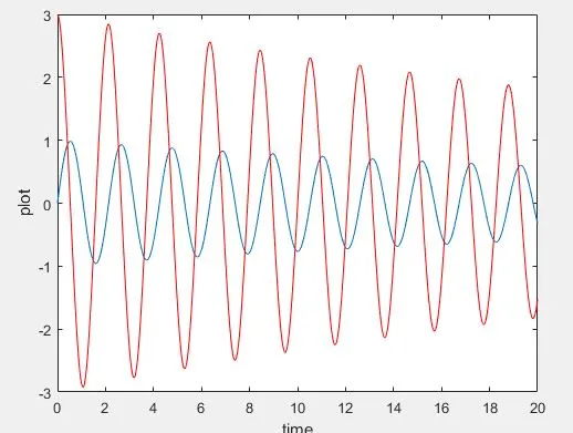
Figure.1

Thus we get the following plot as the output which contains two curves, for a bob of mass 1.0 Kg, Length of the pendulum is 1 metre, & damping coefficient (b) is 0.05. The time period under observation is of 20 seconds, from 0 displacement, & initial angular velocity is 3 rad/sec.

First curve (blue) is for displacement vs time. It starts from 0 & varies from -1 to 1. It depicts how gradually the bob displacement becomes zero, due to damping. The motion has not completely damped yet, as the bob does not come to rest in 20 seconds.

Second curve (red) is for velocity vs time. It shows that the angular velocity starts and varies from 3 to -3 just as we have given as input. Since the motion does not completely damp in 20 seconds the velocity is not zero at the end of the plot.

Now the following video (also in the report) will animate how thw pendulum actually moves under the given time span.

Animation.1

As shown in the graph the motion of the bob does not damp in the given time of 20 seconds, therefore the bob does not come to rest in the end of this video. However the damping of the motion can be clearly seen in the animation as the velocity & displacement of the gradually decrease.

Detailed explanation is given in the report attached