Week 3 - Solving second order ODEs

AIM: To write a program that solves an ODE, representing the equation of motion of a simple pendulum with damping

OBJECTIVES: This project work focuses on solving a second-order differential equation representing the motion of the pendulum. The results are further used to drive a plot of displacement and velocity over time and thus simulating the motion of the pendulum using Matlab. A pendulum is a weight suspended from a pivot so that it can swing freely. When a pendulum is displaced sideways from its resting, equilibrium position, it is subject to a restoring force due to gravity that will accelerate it back toward the equilibrium position. When released, the restoring force acting on the pendulum's mass causes it to oscillate about the equilibrium position, swinging back and forth as shown by the figure below.

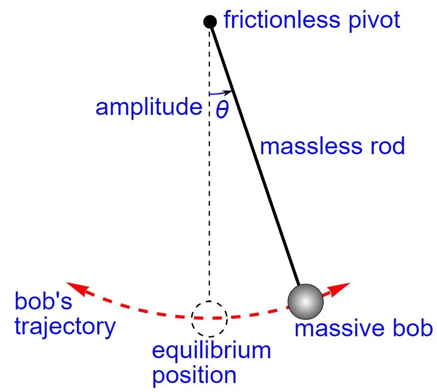
The mathematics of pendulums are in general quite complicated. Simplifying assumptions can be made, which in the case of a simple pendulum allow the equations of motion to be solved analytically for small-angle oscillations. A simple gravity pendulum is an idealized mathematical model of a real pendulum. The model is based on these assumptions

• The rod or cord on which the bob swings is massless and inextensible;
• The bob is a point mass;
• Motion occurs only in two dimensions, i.e. the bob does not trace an ellipse but an arc.
• The loss of energy is only due to damping.
• The gravitational field is uniform.
• The support does not move.

GOVERNING EQUATION: The differential equation which represents the motion of a simple pendulum is:

`(d^2 θ)/dt+ b/m *(dθ)/dt +g/L sin⁡θ=0` ……................Equation 1

Where,

g = gravity in m/s2,

L = length of the pendulum in m,

m = mass of the ball in kg,

b=damping coefficient,

`θ`= angle from the equilibrium position.

For simplification let us convert this second-order differential equation into the first-order differential equation.

Let, `θ=θ_1`…………………………………...........................................….Equation 2

and `(dθ_1)/dt=θ_2`…………………………………...........................……….Equation 3

Now, `(d^2 θ)/dt=(d^2 θ_1)/dt=d/dt ((dθ_1)/dt)=(dθ_2)/dt`…………….. Equation 4

Replacing values of equation 2, 3 and 4 in 1 we have a new equation

`(dθ_2)/dt+ b/m θ_2+g/L sin⁡θ_1=0`………………………..........................….. Equation 5

Hence, the final equations for the motion of pendulum become:

`(dθ_1)/dt=θ_2`………………………......................................................….. Equation 6

`(dθ_2)/dt=- b/m θ_2-g/L sin⁡θ_1`…………………………................................ Equation 7

CODE EXPLANATION: The code is written in Matlab, following is its step-wise explanation:

1. First, all the inputs are assigned their values like damping constant ‘b’ to be 0.05, gravitational constant ‘g’ to be 9.81, length of the string to be 1 meter and mass of bob to be 1 kg.
2. Now a matrix is created by name theta_0, which contains the start values, like time and velocity in separate columns.
3. Now the total time of study is divided into 1000 parts so that differentiation at these values can be done in order to get the best solution
4. Now the function ode45 is used, which is an inbuilt function. This function solves the differential equation using Ranga-Kutta(4,5) methodology. Its syntax is “ [t,y] = ode45(odefun,tspan,y0) ”, where t span = [t0 tf], integrates the system of differential equations y′=f(t,y)from t0 to tf with initial conditions y0. Each row in the solution array y corresponds to a value returned in column vector t.
5. So, parameters are passed in ode45 function such as b, l, g, m, t_span, theta_0 and ‘ode_func’ function giving a matrix of `(dθ_1)/dt` and `(dθ_2)/dt`.
6. In the function ‘ode_func’, parameters are taken, then `(dθ_1)/dt` and `(dθ_2)/dt` are calculated, and assigned to dtheta_dt, which is the output.
7. This result is used by ode45 and solution to this equation are given in the form of results matrix.
8. Now this result containing velocity and displacement are plotted individually with respect to time in a single figure.
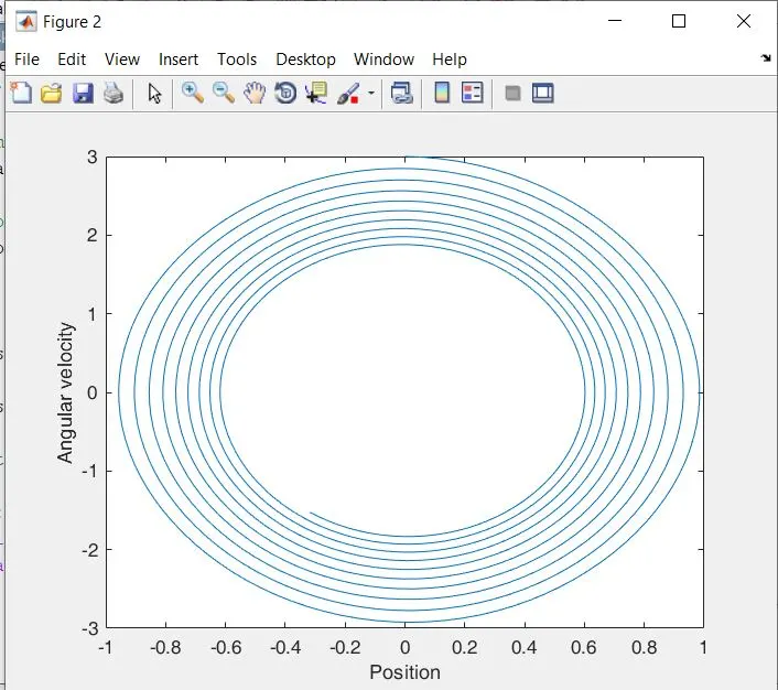
9. Another plot is generated representing velocity corresponding to the position.
10. Now to create an animation for loop is used to extract each frame which runs from i=1 to the length of the result matrix.
11. A counter ct is used to name the frame number, initially assigned a value of 1.
12. Now x0,y0,x1,y1 are defined which are the start and end coordinates of the chord, when a pendulum swings its one end is pivoted or fixed so here x0,y0 is always 0, and x1, y1 varies as the pendulum swings with the given equation, x1= L sin(results), y1= L cos(results).
13. Now the plot for pendulum animation is done, first a blue line of linewidth 2 is drawn which represents the horizontal axis on which one end of the pendulum is pivoted.
14. After that using marker command, a circle is plotted every time on the x1, y1 coordinates representing the circular bob or mass of 1 kg.
15. After this, the string of the pendulum is plotted from x0,y0 to x1,y1.
16. Axis is defined, and the figure is hold off so that plot from every cycle of for loop does not overlap. A hold is used to visualise the movement of the pendulum.
17. Each frame is stored in a matrix M, and ct is the designation of the frame number.
18. Value of ct is updated by adding 1.
19. The loop ends, and these frames are used to create an avi file.
20. Now the frames stored in M are used to generate an animated movie.
21. A video file is created to store this movie in the avi format.
22. After the creation of the file, the file is opened and the frames from M are written in the file and the file is closed.

Here is the main code

clear all
close all
clc
%inputs
%g is gravity in m/s2,L is length of the pendulum in m,m is mass of the ball in kg,b is damping coefficient
b=0.05;
g=9.81;
l=1;
m=1;

%creating a matrix of one row two columns where first is the starting time(0 seconds) and second is the initial velocity(3 m/sec)corresponding to start time
theta_0=[0;3];

% creating a matrix of 1000 values of time span(20 second) 
t_span= linspace(0,20,1000);
 
%using function ode45 and ode_func to solve the diffrential equation by passing parameters
[t, results]=ode45(@(t,theta)ode_func(t,theta,b,g,l,m),t_span, theta_0);

%the solution of diffrentrial equation is used to plot dispacement and velocity
figure(1)
plot(t,results(:,1))
hold on
plot(t,results(:,2))

% another plot is generated to show angular velocity with respect to position
figure(2)
plot(results(:,1),results(:,2))
xlabel('Position')
ylabel('Angular velocity')
axis([-1 1 -3 3])

%to create an animation, different plots are generated and stored in a matrix to get a movie 
%ct is a counter that will store the frame in matrix m for a movie
ct=1;

%the for loop is used to get a frame for every value of displacement result achieved from solving a differential equation
for i=1:length(results(:,1))
    
   %x0,y0 are start point of the chord or string used, 
    x0=0;
    y0=0;
    
    %while x1,y1 are the end points where bob is attached
    x1=l*sin(results(i,1));
    y1=l*cos(results(i,1));
    
    % A plot is genrated showing the mass, string and the fixed pivot line.
    figure(3)
    % the blue line is a staight line having piviot point of string 
    plot([-1 1],[0 0],'linewidth',2,'color','b')
    hold on
    % now on points x1,y1 the bob is represented using a marker
    plot(-x1,-y1,'-O','MarkerSize',15,'MarkerEdgeColor','red','MarkerFaceColor','r')
    % the plot of the string is now done between x0,x1 and y0,y1. x1 and y1 are taken negative so as the mass hangs below the pivot line
    plot([-x1 x0],[-y1 y0],'linewidth',2,'color','r')
    axis([-1.5 1.5 -1.5 0.5])
    %To have a visible moving plot a pause is used
    pause(0.003)
    hold off
    %storing this plot frame in a mattrix M
    M(ct)=getframe(gcf);
      ct=ct+1;
end
%creating a movie or avi file using the frames stored in M
movie(M)
videofile= VideoWriter('Pendullam_motion.avi','Uncompressed AVI');
open(videofile)
writeVideo(videofile,M)
close(videofile)

Here is the code for a function used ode_func

%ode function representing the simplified equation for the motion of the pendulum

function[dtheta_dt]=ode_func(t,theta,b,g,l,m)
% all the required parameters are passed

% the second order equation is converted into single order using a another variable theta2
% let theta=theta1, and (d theta1)/dt= theta2, so new equations are

theta1=theta(1)
theta2=theta(2)

%providing the equations and storing their result in a 2 column matrix

dtheta1_dt= theta2;
dtheta2_dt=-(b/m)*theta2-(g/l)*sin(theta1);
dtheta_dt=[dtheta1_dt;dtheta2_dt]


end

ERRORS FACED: This solution wasn’t achieved in the first attempt, a few errors were faced achieving the end result, which are as follows:

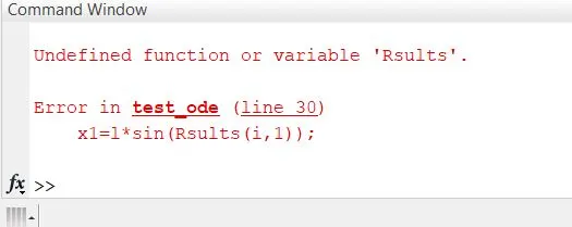
• My first error was a silly typing error, as shown below. I corrected it easily.

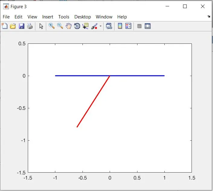
• My error was a syntax error for marker representing the mass, it took a lot of time to figure out, but checking syntax online helped me overcome it.

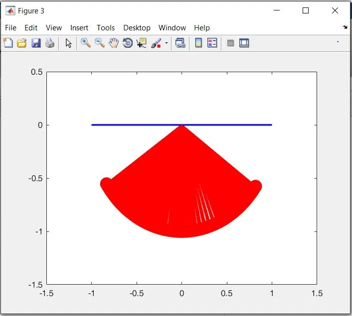
• A different error as shown below was that I was not able to see every plot of animation differently, instead, the plots were overlapping. After researching the use of hold off command before the end of the for loop helped me sort this problem.

• I was getting the animation for the figure I declared for the different plot, this made me think to assign animation a different figure.

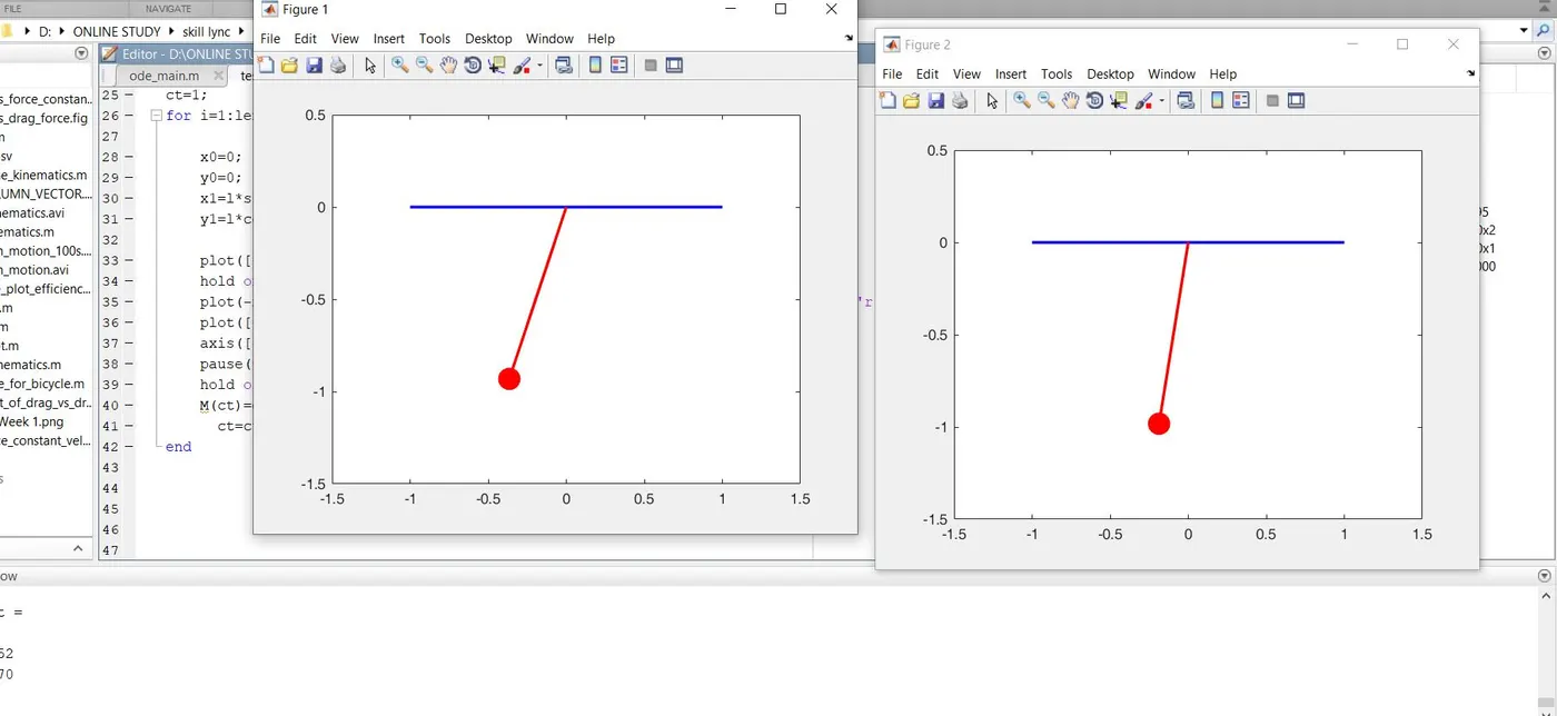
• One of the most problematic errors I faced was that my pendulum was inverted, It took a lot of time to understand that my x1 and y1 coordinates are in the positive y-direction. Then to overcome it I placed a ‘-‘ sign before x1 and y1 so that my pendulum looks downward.

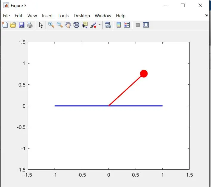
Results and Conclusion: After facing different errors, my concepts and use of MatLab got stronger. I was able to plot the solution of a differential equation representing the motion of a pendulum, shown below.

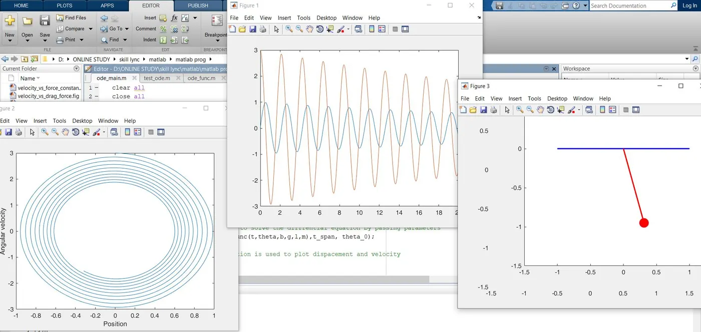
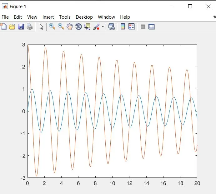
The figure below is my first plot which shows the solution differential equation with respect to time, here red curve is the velocity solution and the blue curve is the displacement solution.

The second plot was the plot of angular velocity with respect to the position; i.e. from this curve at any instance velocity and corresponding displacement can be determined.

My final plot was to create an animation, Here is the link to my animated video

https://youtu.be/Y6Kz2hnzxD8

THANK YOU